How do you turn massive infrastructure and cultural datasets into clear visual stories?
Most public data projects stall right after the first download. An analyst pulls an API dump of global network routes or millions of daily web logs, opens a blank chart canvas, and gets stuck. The raw file is full of duplicate entity names, shifting date formats, and extreme outliers that flatten every visual scale.
Turning massive public logs or internal tables into a readable narrative takes a disciplined pipeline before you pick a chart type. Whether you are mapping physical hardware on the ocean floor or measuring what millions of people read and listen to, the raw rows rarely match the real-world concepts your audience cares about.
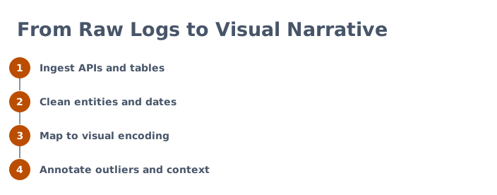
- Ingest APIs and tables: Pull structured records from public endpoints, geospatial files, or historical spreadsheets while preserving raw identifiers.
- Clean entities and dates: Standardize subsidiary names, resolve corporate mergers, and align shifting calendar intervals into a consistent time grain.
- Map to visual encoding: Assign cleaned variables to spatial coordinates, color scales, or ranked positions that reflect the real structure of the data.
- Annotate outliers and context: Layer human explanations directly onto major spikes, structural breaks, and missing records so readers understand why the numbers moved.
How is global submarine cable data structured and mapped?
TeleGeography confirms that submarine cables carry more than 99% of intercontinental data traffic. In the visual investigation of Big Tech undersea cables, the dataset covers 712 active, planned, and retired submarine systems from TeleGeography's public Submarine Cable Map database (API v3), combined with Natural Earth land boundary data.
For most of the internet's history, telecom carriers built and owned these systems in large consortiums, while technology firms simply rented capacity.
Structuring this dataset requires linking route geometry to ownership arrays and ready-for-service (RFS) years. Across the 712 systems, 62 list Google, Meta, Amazon, or Microsoft among their owners, and 27 of those Big Tech cables are planned or under construction.
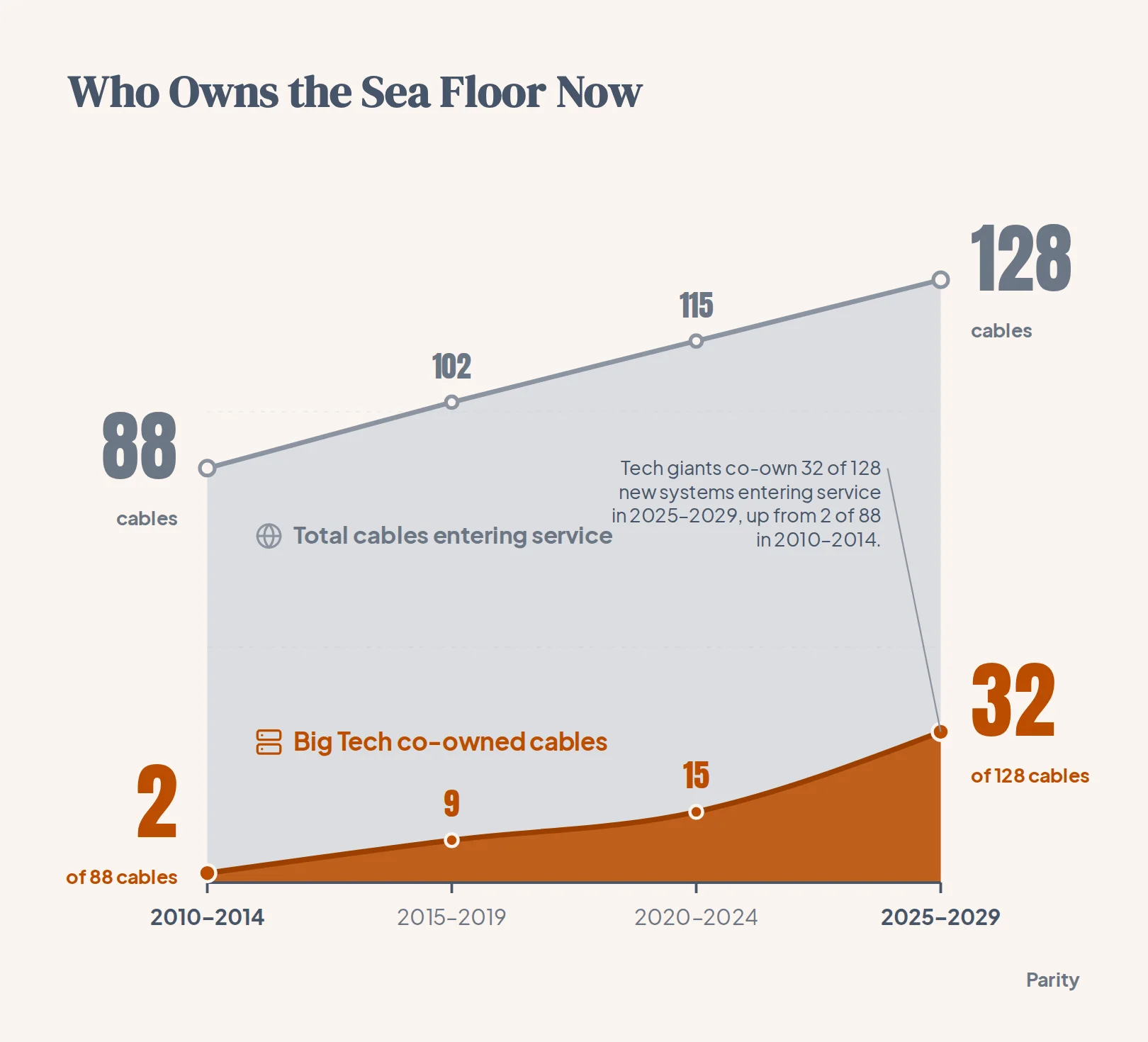
Only 2 of the 88 cables entering service from 2010 to 2014 had one of the four companies as an owner, rising to 9 of 102 in 2015 to 2019, 15 of 115 in 2020 to 2024, and 32 of the 128 cables due from 2025 to 2029 (25%).
To make these patterns legible on a dark canvas, the visual encoding separates the background network from the four major cloud builders and breaks down their distinct footprints:
- Visual hierarchy on the map: Non-Big Tech systems are drawn as faint grey lines, while cables owned by the four companies glow in each company's color and dashed lines mark cables co-owned by two of them.
- Meta: Co-owns 21 cables in the database, including the 45,000 km 2Africa loop around Africa, and announced Project Waterworth in February 2025 to span more than 50,000 km across five continents.
- Microsoft and Amazon: Microsoft co-owns 8 cables and Amazon co-owns 6, frequently partnering on joint routes like Beaufort, JAKO, and Asia United Gateway East, alongside Amazon's 320+ terabits per second Fastnet cable (announced November 2025, due in 2028 between Maryland and County Cork, Ireland).
What data cleaning challenges come up when mapping physical networks?
Physical infrastructure records look tidy in an API response, but mapping them accurately requires resolving real-world ambiguities. In the TeleGeography database, the 712 systems have listed lengths totaling about 1,973,000 km (with Big Tech cables accounting for about 529,000 km), whereas TeleGeography reports about 1.5 million km of cable actually in service in early 2026 and headlines "more than 600 active and planned" cables.
That gap exists because raw infrastructure databases mix active hardware, retired cables, and multi-year construction plans. Deep-water cables are thinner than a garden hose, cost $6,000 to $20,000 per kilometre plus roughly $200,000 per optical repeater every 50 to 100 km, and run around $250 million for a 7,000 km transatlantic crossing or up to $400 million across the Pacific.
Because a single new cable can carry hundreds of terabits per second (contributing to global used international bandwidth of more than 6.4 petabits per second in 2025), cloud providers build redundant paths to avoid chokepoints.
Physical vulnerability makes route diversity a major theme in the data. In February 2024, Red Sea cable cuts affected about a quarter of regional traffic, and another Red Sea cut in September 2025 forced Microsoft's Azure cloud to reroute Asia-Europe traffic and warn of higher latency.
When cleaning physical network tables for visual analysis, analysts have to handle several recurring data anomalies:
- Slipping future dates: Because 27 of the 62 Big Tech cables have RFS dates in 2026 or later, construction schedules can slip and planned routes (such as Meta's Project Waterworth) may not have geometry drawn yet.
- Entity name changes: Historical entries may list legacy corporate names such as Facebook alongside Meta, requiring entity resolution rules before grouping.
| System Name | Listed Length | Tech Co-Owners | RFS Year (State) |
|---|---|---|---|
| Amitie | 6,792 km | Meta, Microsoft | 2023 (In service) |
| Topaz | Unlisted | 2023 (In service) | |
| 2Africa | 45,000 km | Meta | 2024 (In service) |
| Apricot | 11,972 km | Google, Meta | 2025 (In service) |
| Bulikula | 21,600 km | 2026 (Planned) | |
| Tabua | Unlisted | 2026 (Planned) | |
| Beaufort | 158 km | Amazon, Microsoft | 2027 (Planned) |
| Raman | 7,376 km | 2027 (Planned) |
How do you clean and visualize Wikipedia traffic data to measure cultural attention?
While undersea cables show where physical capacity sits, encyclopedia traffic logs reveal what people actually look up.
Even when you filter for human readers rather than web crawlers, stealth scrapers, uptime monitors, and default browser homepages generate millions of artificial hits across desktop and mobile channels that distort cultural rankings.
Tip: Always compare desktop and mobile web view shares when auditing top Wikipedia pages. Genuine human curiosity almost always shows a balanced split across both platforms, whereas an article with lopsided desktop or mobile app views is nearly always the byproduct of an automated script or a preloaded software widget.
To isolate genuine human attention from technical noise, your transformation pipeline needs four specific cleaning steps:
- Strip navigation and namespace pages: Filter out
Main_Page,Special:Search,Special:CreateAccount, and internalWikipedia:orPortal:namespaces that capture portal navigation rather than reading. - Consolidate article redirects: Merge traffic from URL variants, punctuation differences, and renamed page titles into the canonical article identifier so views are not split across duplicates.
- Flag single-platform bot anomalies: Exclude pages where traffic spikes occur almost entirely on a single access channel without corresponding search or mobile readership.
- Group into thematic categories: Tag cleaned articles by topic (such as elections, sports tournaments, film releases, and obituaries) so the visual layout separates sudden news spikes from steady year-round reference staples.
How do you structure 68 years of Billboard Hot 100 number one hits for visual analysis?
Long-running cultural rankings introduce a different problem: the rules of the measurement change while the chart keeps running.
Furthermore, artist credit strings grow significantly messier over time as solo credits give way to multi-artist collaborations (Artist A Featuring Artist B & Artist C).
Preparing a multi-decade chart archive for visual storytelling requires resolving three structural hurdles:
- Normalize featured artist credits: Split compound credit strings into a relational bridging table so collaborations count properly toward each performer's career total without double-counting the week.
- Track non-consecutive runs: Group chart weeks by a unique song identifier alongside a run sequence number so tracks that drop off the top spot and return months or years later (such as holiday perennials) are measured accurately.
- Annotate methodology eras: Mark major rule changes directly on timeline axes (such as the introduction of electronic sales data or the integration of streaming) so readers do not mistake measurement changes for organic shifts in listener behavior.
| Dataset | Primary Key | Main Cleaning Challenge | Best Visual Encoding |
|---|---|---|---|
| Submarine fiber cables | System ID and RFS year | Consortium co-ownership and future dates | Geospatial route map and dot timeline |
| Wikipedia pageviews | Canonical article title and date | Portal pages and single-platform bot spikes | Ranked bar chart and daily sparklines |
| Billboard Hot 100 #1s | Chart week date and song ID | Multi-artist credits and rule changes | Era timeline and streak barcode chart |
How can you build checked dashboards and reports from your own spreadsheets?
Public investigations take days of custom scripting, entity resolution, and layout tuning, but business teams need that same numerical rigor for their weekly operational files in minutes.
When you connect a spreadsheet or any of 54 supported business tools, Parity automatically builds an interactive dashboard and uses its AI report generator to turn raw data into formatted reports with executive summaries, charts, tables, and written analysis in seconds, checking every number against your source data.
You can click any headline number to inspect the underlying queries and counted rows, chat with plain-English prompts to refine charts, follow next move suggestions on what to look at next, and export presentation-ready PDFs with a single click on either Cloud Hosted infrastructure or an on-premise Local Mac Mini.
Connect a spreadsheet or the tools you run on, and Parity builds the interactive dashboard and writes the formatted report with every number checked against your source data. Build a report from your data free