Why do VLOOKUP and SUMIFS totals mismatch across monthly tabs?
Here is a routine most operations and finance leads know by heart: a workbook with monthly tabs of invoice exports, a summary sheet stitched together with SUMIFS, and a lookup table pulling customer regions via VLOOKUP. The summary chart says revenue dipped in November, while the accounting ledger says it rose. Both numbers came from the same month's exports.
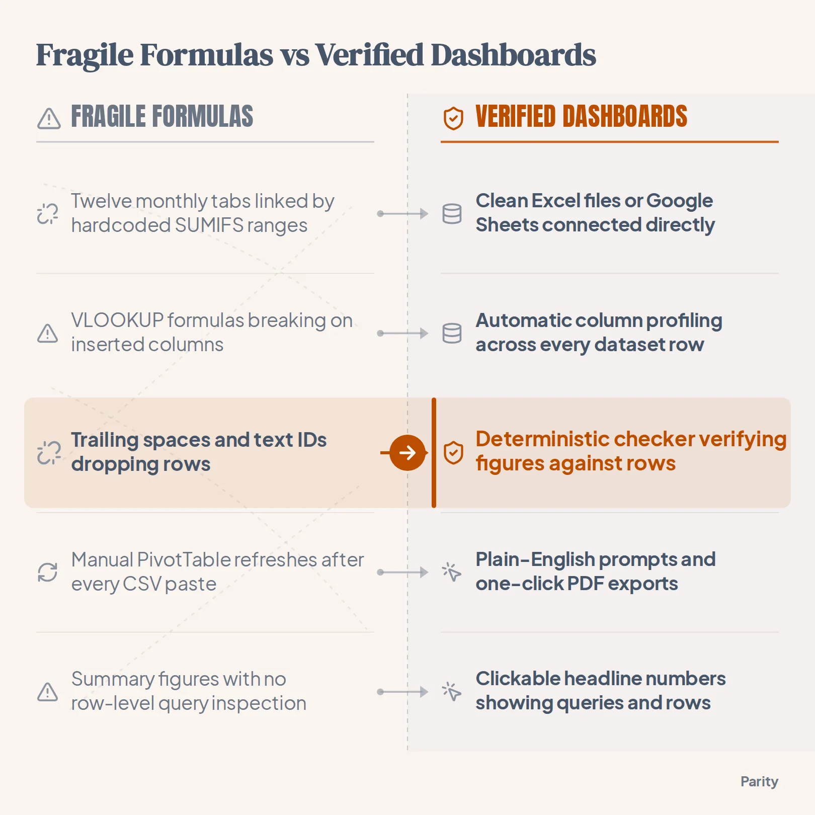
The summary sheet missed a batch of rows because November's export was longer than October's static range, and several customer IDs came in formatted as text instead of numbers. A spreadsheet formula only calculates against the exact cell coordinates and data types it is given. When each month lives on its own tab, small structural drift between tabs causes formulas to drop rows without displaying an #N/A or #VALUE! warning.
Microsoft's VLOOKUP function documentation notes that VLOOKUP requires the lookup value to sit in the leftmost column of the table array and relies on a hardcoded column index number. Meanwhile, the official SUMIFS function reference specifies that every criteria_range must contain the exact same number of rows and columns as the sum_range.
When you copy tabs from month to month, four failure modes routinely distort your totals behind the scenes. If you are already troubleshooting a broken sheet, compare these patterns with our guides on Excel dashboard templates and moving from Excel pivot charts and invoice PDFs to live AI dashboards.
| Failure mode | What happens in the tab | Effect on VLOOKUP | Effect on SUMIFS | Visible error flag? |
|---|---|---|---|---|
| Trailing or leading spaces | Exported CRM or ERP strings include a hidden space after the ID or category name | Returns #N/A unless wrapped in TRIM, dropping the row from downstream sums | Excludes the row from the criteria match and under-reports the total | VLOOKUP shows #N/A; SUMIFS fails silently |
| Text vs. number IDs | One month stores SKU or account IDs as text strings, while the lookup table stores integers | Fails to match the key and returns #N/A | Automatically coerces numeric strings in some cases, or skips mismatched keys | VLOOKUP shows #N/A; SUMIFS fails silently |
| Inserted columns | An analyst adds a 'Notes' or 'Discount' column in the middle of March's tab | Hardcoded col_index_num pulls from the shifted column instead of the target field | Unaffected if column letters shift dynamically, breaks if referenced by indirect text | Fails silently (pulls wrong column) |
| Shifted range boundaries | April has more rows than March, exceeding the static A2:G500 formula range | Ignores any new lookup keys added below the static table boundary | Omits all transactions below row 500 or returns #VALUE! if ranges differ in length | Fails silently when both ranges stop short |
What you need
Before you overhaul a fragile multi-tab workbook, gather the raw files and access you will use to build a clean pipeline. You do not need database credentials or BI modeling tools to get started.
- Your source spreadsheet: An Excel workbook (
.xlsxor.xls), CSV export, or multi-tab Google Sheet containing your historical and current period rows. - Consistent business keys: One identifier per entity, such as Customer ID, Invoice Number, or SKU, that appears on every tab you plan to combine.
- Source ledger totals: One known control figure from your accounting or commerce system, such as monthly gross revenue or total orders, to verify your final dashboard.
- A Parity account: Access to the Excel to dashboard tool or the spreadsheet and tool connectors to read your sheets and verify the math.
1. Audit and standardize column headers and key types across tabs
Whether you plan to consolidate tabs inside a spreadsheet or upload your workbook to an automated generator, your columns need consistent names and formats. When January calls a column Client_ID and February calls it Customer #, any automated query or formula has to guess whether they represent the same field.
Start by inspecting the top rows and key columns of every monthly tab in your workbook. According to Google's VLOOKUP function help page, Google recommends setting is_sorted to FALSE so an exact match is returned unless your search key column is sorted in ascending order.
Run through this four-part cleanup across your tabs before combining them:
- Unban merged title cells: Delete decorative banner rows at the top of each tab so row one is a single, flat header row with one label per column.
- Strip hidden whitespace: Apply
TRIMandCLEANto text keys, category labels, and regional tags so trailing spaces from CSV exports do not split one category into two. - Lock data types on IDs and dates: Format invoice numbers, SKUs, and account codes consistently as either text or integer across every tab, and convert regional text dates into standard ISO dates (
YYYY-MM-DD). - Remove inline subtotal rows: Delete manual 'Total' or 'Q1 Subtotal' rows embedded in the middle or bottom of raw data tabs so summary queries do not double-count your revenue.
Watch out: Never leave an approximate match default (
TRUEor omitted) in aVLOOKUPformula across monthly tabs. If a new customer ID is missing from the lookup tab, an omitted fourth argument forces the spreadsheet to grab a neighboring row's value instead of flagging a missing key.
2. Consolidate monthly tabs into a single flat table or clean workbook
The most common mistake in spreadsheet reporting is treating a time period as a tab name rather than a column value. When 'January 2026', 'February 2026', and 'March 2026' only exist as worksheet labels at the bottom of the screen, you cannot filter, group, or trend across the quarter without writing complex INDIRECT formulas or daisy-chained SUMIFS blocks.
Instead of writing cross-tab cell references that reach into twelve separate sheets, structure your workbook so every transaction row carries its own date or period column. Combining uniform monthly tables into a single flat table keeps new rows inside the calculation boundary automatically.
Choose one of these three ways to organize your multi-tab file:
- Append rows with a Period column: Stack your monthly exports into one master transactions tab where Column A records the transaction date or reporting month.
- Keep tidy raw tabs with identical headers: If you prefer keeping one tab per month or per department in Google Sheets or Excel, make sure every tab uses the exact same header row and includes a date column on every line.
- Separate lookup tables from transaction logs: Keep customer metadata, product cost tables, or regional mappings on one dedicated reference tab rather than pasting redundant columns into every monthly sheet.
3. How do you combine multiple spreadsheet tabs into a live dashboard without broken formulas?
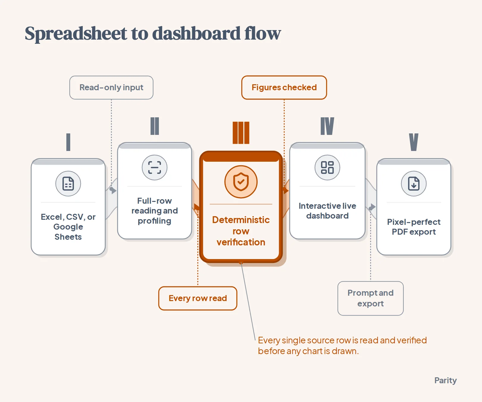
Once your workbook has tidy headers, you can skip manual pivot tables and cross-tab formulas altogether. With Parity's AI dashboard generator, you upload an Excel (.xlsx or .xls) or CSV file, or connect Google Sheets to read any sheet and every tab.
You can also connect Google Drive, Excel on OneDrive, or Airtable, or pull directly from any of the 54 supported tools including QuickBooks, Stripe, and Shopify. When you drop in a file or connect a sheet, Parity reads every row across the full dataset rather than taking a sample, profiles the columns automatically, and builds an interactive dashboard in a few minutes.
Follow these steps to turn your multi-tab sheet into a live dashboard:
- Connect or upload your data: Upload one or several Excel or CSV files, or link your Google Sheets, Google Drive, or Excel on OneDrive account in read-only mode.
- Describe what you want to see: Type a plain-English prompt naming the metrics, trends, and category breakdowns your team tracks each month.
- Let Parity profile the full dataset: Parity reads every row, selects the charts, KPI cards, and tables, and writes plain-English analysis explaining the trends.
4. Verify every headline figure against the underlying source rows
A dashboard is only useful if finance and operations leads can trust the math in a review meeting. In a traditional spreadsheet, auditing a questionable total means clicking into a cell, tracing precedents across tabs, and checking whether a SUMIFS range stopped forty rows above the bottom of the sheet.
Parity removes manual formula tracing with a deterministic checker. Before any dashboard or report is shown on screen, the deterministic checker recomputes every figure against the underlying source rows in your dataset, fixing or flagging anything that does not match.
Use these three checks to validate your dashboard before sharing it with stakeholders:
- Click the headline numbers: Click any top-level summary metric on your Parity dashboard to inspect the exact query behind it and view the source rows it counted.
- Confirm full-row coverage: Check the row counts on your inspected queries against your raw export totals to confirm that every charge, invoice, or order across your tabs was included.
- Review the plain-English drivers: Read the written analysis alongside each trend chart to see what explains the month-over-month change and what Parity suggests asking next.
5. Refine breakdowns in plain words and roll the dashboard forward each month
In a multi-tab Excel workbook, answering a follow-up question from an executive or client usually means inserting a new helper column, rewriting a SUMIFS block across twelve tabs, and rebuilding a chart by hand. In Parity, you refine your dashboard and reports by chatting in plain words.
When you ask for a new chart, a different regional breakdown, or a revised summary, the dashboard updates in place and re-runs the numbers against your data. Every change is saved as a version you can step back to, so experimenting with a new view never puts your verified layout at risk.
When the next reporting cycle arrives, you do not have to rebuild formulas from scratch:
- Re-run on the new period's data: Upload the new month's spreadsheet or refresh your connected sheet to keep a consistent layout across reporting cycles.
- Customize sections by prompt: Use plain-English prompts to highlight specific variances or add a table before sending the report to clients or leadership.
- Export a pixel-perfect PDF: Export your finished dashboard or client-ready report as a PDF in one click that looks exactly as it appears on screen.
Upload an Excel or CSV file or connect Google Sheets and 54 business tools. Parity reads every row, checks every figure against your data, and exports a pixel-perfect PDF. Build your dashboard free