What you need
How do you chart half a century of monthly state unemployment records without drawing an unreadable tangle of overlapping lines? An analyst downloads the historical labor table and plots every state on a single time axis. Extreme crisis spikes flatten normal business cycles, while dozens of regional trajectories disappear into a dense ribbon of ink.
Before you plot the Bureau of Labor Statistics (BLS) series, gather these core inputs:
- BLS LAUS bulk files or API access: Access the Local Area Unemployment Statistics database via the public JSON API or flat text files.
- FIPS state and Census division lookup table: A reference file mapping two-digit state codes to the nine official US Census Bureau divisions.
- Data preparation environment: Python, R, SQL, or a spreadsheet workflow capable of parsing fixed-width series identifiers and pivoting wide matrices.
- Preparation time: Roughly thirty minutes to filter seasonal flags, verify denominator columns, and configure a non-linear color scale.
1. Why 50 years of monthly state unemployment data breaks standard line charts
When you pull monthly unemployment rates for all fifty states plus the District of Columbia from the start of the modern state series in 1976, you get over thirty thousand monthly observations. Plotting fifty-one continuous series across five decades on a standard Cartesian line chart creates immediate visual failure.
Three structural properties of state labor markets cause standard line charts to fail:
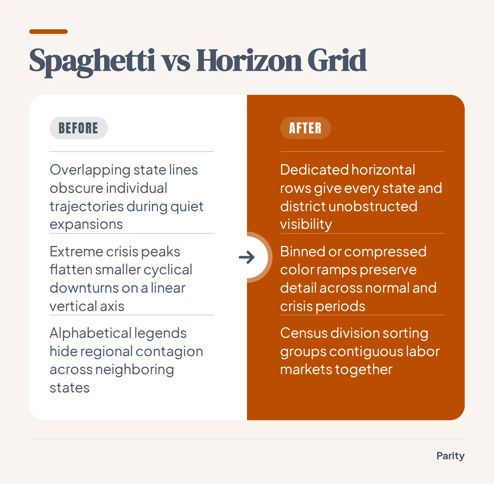
- Expansion band overplotting: Most states cluster inside a narrow band of low single-digit rates during economic expansions, turning the middle of the canvas into an unreadable braid where individual paths cannot be traced.
- Extreme shock compression: Sudden national lockdowns or severe regional industrial downturns push individual state rates far above normal ranges, forcing a linear vertical axis to compress mild recessions into flat lines.
- Missing geographic adjacency: Alphabetical legends scatter neighboring states across the color palette, hiding how economic shocks spread across contiguous regions.
Replacing overlapping strokes with spatial matrices or folded bands solves these problems at once. You give every jurisdiction its own dedicated horizontal track while preserving exact chronological alignment across the entire historical record.
2. How the BLS Local Area Unemployment Statistics (LAUS) dataset is structured
When you query the BLS Public Data API or download flat files from the LAUS program, records are indexed by a standardized twenty-character string called the series identifier. Parsing this identifier cleanly is the fastest way to filter state-level panels without joining multiple metadata tables.
Every LAUS series identifier follows a strict positional grammar:
- Survey prefix (positions 1 to 2): Always
LAfor Local Area Unemployment Statistics. - Seasonal adjustment code (position 3): Marked as
Sfor seasonally adjusted series orUfor unadjusted raw estimates. - Area code (positions 4 to 18): A fifteen-character geographic string starting with
STfor states, followed by the two-digit state FIPS code and eleven trailing zeros. - Measure code (positions 19 to 20): A two-digit suffix indicating whether the series measures the unemployment rate, unemployed count, employed count, or civilian labor force.
Always pull all four measure codes when building an analytical table. Storing the underlying headcount columns alongside the pre-calculated rate allows you to compute exact population-weighted regional aggregates later without averaging percentages across states of vastly different population sizes.
| Segment | Positions | Code Values | Definition |
|---|---|---|---|
| Survey Prefix | 1 to 2 | LA | Local Area Unemployment Statistics program |
| Seasonal Code | 3 | S or U | Seasonally adjusted (S) or unadjusted (U) |
| Area Type & FIPS | 4 to 18 | ST + FIPS + zeros | State area code with two-digit state FIPS |
| Unemployment Rate | 19 to 20 | 03 | Unemployed percentage of labor force |
| Unemployment Count | 19 to 20 | 04 | Total unemployed persons in state |
| Employment Count | 19 to 20 | 05 | Total employed persons in state |
| Labor Force Count | 19 to 20 | 06 | Total civilian labor force count |
3. Seasonal adjustment, benchmark revisions, and cleaning rules before you plot
Raw public labor files contain summary rows, seasonal swings, and retroactive methodology updates that can corrupt a multi-decade chart if plotted directly. Run four validation checks on your extracted table before binding it to a visual canvas:
- Separate
LASfromLAUrecords: Never mix seasonally adjusted (LAS) and unadjusted (LAU) series in the same chart. Unadjusted state numbers spike every January after holiday retail contracts end and every June when schools close, creating vertical stripes on a monthly heatmap. - Filter out
M13annual averages: BLS flat files include a thirteenth period (M13) representing the annual average alongside monthsM01throughM12. LeavingM13in a chronological time series injects an artificial thirteenth month at the end of every calendar year. - Exclude non-state territories for balanced panels: Filter your area codes to the fifty states and Washington, D.C. (
ST01throughST56, excluding reserved FIPS gaps) if you require a complete historical matrix starting from January 1976. - Replace cached tables after annual benchmarking: Each spring, the BLS revises recent years of state estimates to incorporate updated population controls and unemployment insurance tax records. Always overwrite your full historical table rather than appending only the latest month.
Watch out: Never compute a multi-state regional unemployment rate by taking the simple arithmetic mean of state rates. Always sum the unemployed headcount (
04) across all states in the region and divide by the summed civilian labor force (06) so populous states like California and Texas receive accurate weight.
4. Four ways to chart 30,600 monthly state records without clutter
Once your panel is cleaned, choose a visual encoding that matches the question your reader is asking. When mapping fifty years of state-level housing records in our US home prices by state story, arranging all 51 spokes by Census region across 202 quarterly rings made 10,302 cells readable by color alone. You can apply the same dense encoding principles to monthly unemployment panels using four layouts:
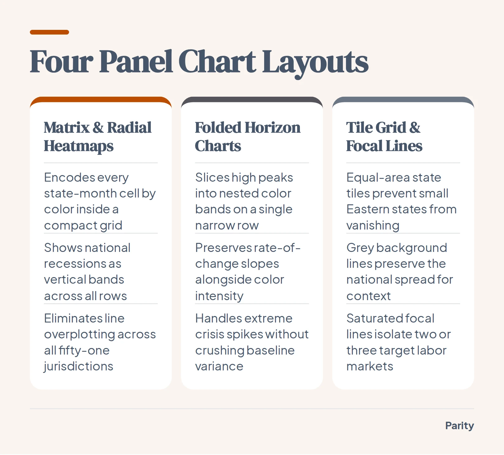
- Matrix and radial heatmaps: Map time along the horizontal axis (or concentric rings) and states along the vertical axis (or radial spokes), encoding the monthly unemployment rate by color hue and luminance. National recessions appear immediately as vertical bands cutting across all rows, while regional slumps show up as localized horizontal streaks.
- Horizon charts: Slice each state's area chart into uniform horizontal elevation bands and layer darker color steps onto a single compact track. Horizon charts preserve line-slope intuition while reducing vertical row height enough to fit all fifty-one jurisdictions on one screen without scrolling.
- Small multiples on a US tile grid: Place fifty-one miniature line or area sparklines inside an approximate geographic grid where every state occupies an equal square. Tile grids reveal spatial contagion across borders while preventing geographically small states like Rhode Island and Delaware from disappearing.
- Grey context spaghetti with focal callouts: When a stakeholder insists on a traditional line chart, draw all background states in low-opacity neutral grey, add a dashed line for the national median, and highlight only two or three focal states in saturated color.
5. Handling the April 2020 scale problem: when a single shock dwarfs 50 years of history
Every multi-decade unemployment visualization hits a severe scaling obstacle in the spring of 2020. During the initial pandemic lockdowns, service and hospitality hubs like Nevada, Michigan, and Hawaii saw monthly jobless rates surge to historic highs that far exceeded any prior postwar recession. Before 2020, only a few industrial states had ever reached comparable territory during the early 1980s downturn.
If you bind a sequential color ramp linearly from the historical minimum to the April 2020 peak, almost the entire fifty-year matrix sits in the bottom half of your palette. Moderate recessions lose visual contrast and blend into the baseline.
6. What five decades of state joblessness data reveal when sorted by region
Sorting the vertical axis alphabetically puts Alabama next to Alaska and Wyoming at the bottom, breaking up contiguous economic zones. Grouping rows by the nine official US Census divisions and ordering states within each division by their long-term median rate turns random horizontal noise into coherent geographic blocks.
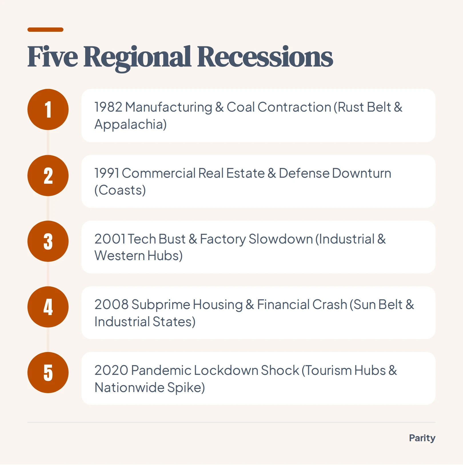
- Early 1980s industrial recessions: Deep dark bands concentrate in the East North Central and East South Central manufacturing and coal belts, led by Michigan and West Virginia.
- Mid-1980s energy and farm bust: Even as coastal economies recover, elevated joblessness lingers across West South Central and Mountain oil states.
- 2015 shale oil downturn: A localized ripple of rising unemployment hits North Dakota, Wyoming, West Virginia, and Oklahoma while the rest of the country continues expanding.
- Spring 2020 pandemic shock: A sharp vertical wall of high joblessness hits almost every row simultaneously in April 2020, followed by a rapid recovery in inland agricultural states and a slower rebound in tourism hubs.
7. Building checked dashboards and reports from public BLS data and your own spreadsheets
Exploring public economic records is much faster when the data and visual encodings are already assembled. On our public data stories hub, you can browse 64 graphics built from open datasets including the BLS, World Bank, NOAA, NASA, UNHCR, and the US Treasury, and download any chart or its underlying data to use with credit, including our BLS grocery receipt price comparison.
Every headline figure is verified against the dataset so you can click a number to inspect the underlying calculation queries and counted rows, adjust charts with conversational natural language prompts, and export presentation-ready PDF files with a single click.
Connect a spreadsheet or the tools you run on, and Parity builds an interactive dashboard and writes the report in minutes with every number checked. Build a report from your data free