Charts like this, from your own numbers.
Connect a spreadsheet or the tools you run on, and Parity builds the dashboard and writes the report, with every number checked.
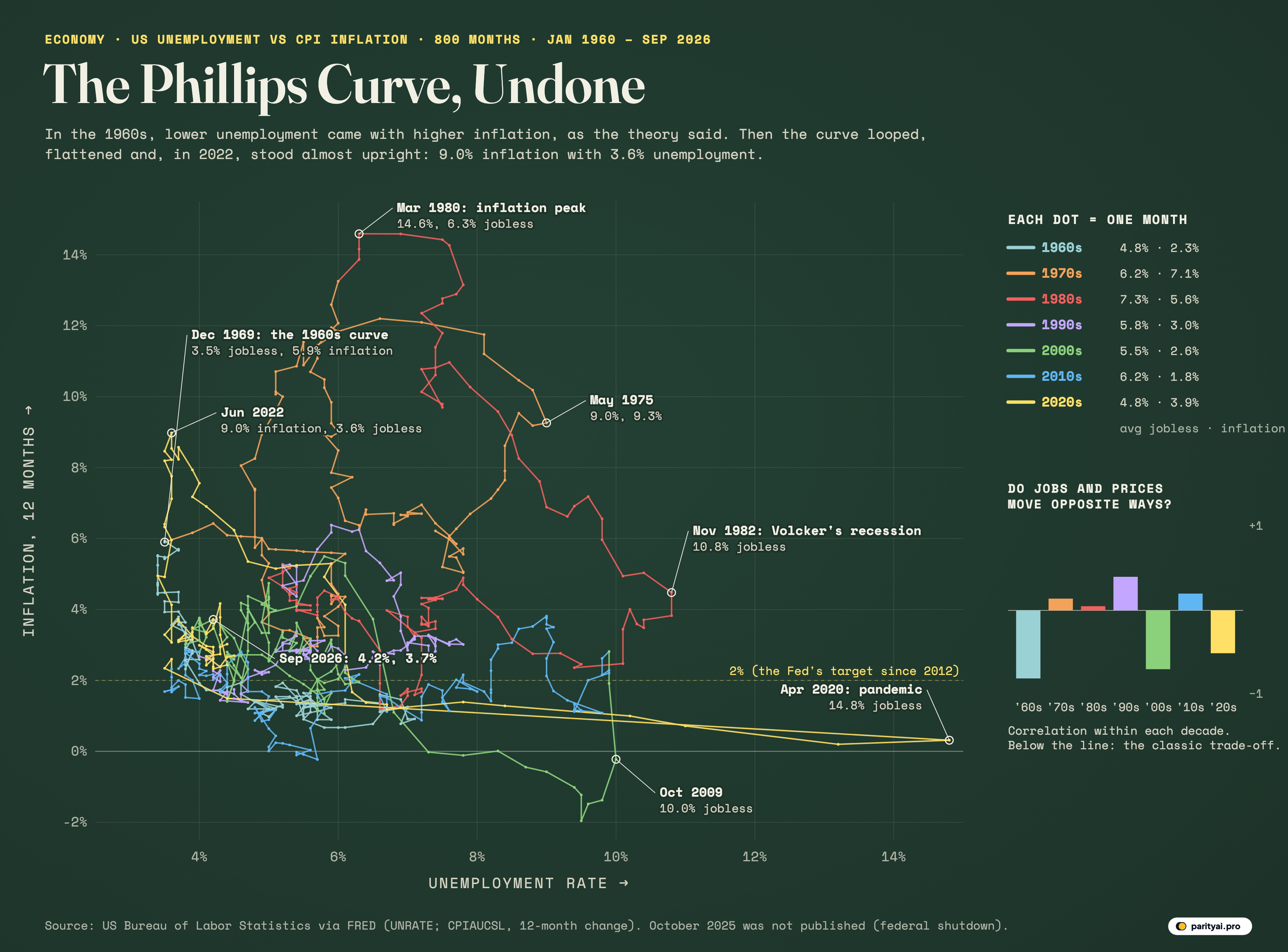
Try Parity freeIn June 2022, American consumer prices were 9.0% higher than a year earlier, on the seasonally adjusted measure plotted here, while the unemployment rate was 3.6%. The Bureau of Labor Statistics called the headline figure, 9.1% before seasonal adjustment, the largest 12-month increase since the 12-month period ending November 1981. Ten months later, unemployment fell to 3.4%; the BLS noted that only one other month since May 1969 had seen it below 3.5 percent.
High inflation with very low unemployment is what an old idea in economics, the Phillips curve, would predict. The idea is that the two trade off: when jobs are plentiful, prices rise faster; when unemployment is high, inflation cools. For much of the past half-century, though, the data have seemed to ignore it.
The chart above puts the idea on trial. Each of its 800 dots is one month from January 1960 to September 2026. Its position across is that month's unemployment rate; its height is inflation over the previous 12 months, measured by the consumer price index. A line joins each month to the next, coloured by decade, so the path shows how the economy moved. If the Phillips curve held perfectly, every dot would sit on one downward-sloping line from top left to bottom right.
The evidence comes in exhibits, decade by decade.
Exhibit A: the curve as advertised (the 1960s)
The idea began in 1958, when the economist A. W. Phillips examined U.K. unemployment and wages from 1861 to 1957 and found an inverse relationship between the level of unemployment and the rate of change in wages. Two years later, Paul Samuelson and Robert Solow recast it for the United States in terms of prices, and were the first to treat it as a menu for policy: choose a little more inflation and buy a little less unemployment.
The pale blue path of the 1960s, at the left of the chart, is the curve as advertised. Unemployment started the decade at 7.1% in May 1961 and fell steadily to 3.4% in September 1968; inflation rose from 0.7% to 5.9% by November 1969. Within the decade, the correlation between the two is -0.81, strongly negative, as the theory says. By December 1969 the path had reached its tightest point: 3.5% unemployment and 5.9% inflation.
Exhibit B: the loops (the 1970s and early 1980s)
Then the path breaks free. The orange and red lines of the 1970s and early 1980s climb up and to the right, then loop back, in great arcs that cover most of the chart. In May 1975 unemployment reached 9.0% with inflation at 9.3%: both high at once. The Federal Reserve's own history of the period calls it the era of 'stagflation'.
Within the 1970s the correlation between unemployment and inflation is 0.14, essentially zero. The trade-off had vanished. In his presidential address to the American Economic Association, delivered in December 1967 and published in March 1968, Milton Friedman had warned that the trade-off would not last; Gregory Mankiw and Ricardo Reis later called the lecture a turning point in the history of macroeconomic research. Once people expect inflation, the argument goes, they build it into wages and prices, and the curve shifts up. The Fed's history is blunt on the point: "Phelps and Friedman were right."
The top of the chart is March 1980, when inflation on this measure peaked at 14.6%, with unemployment at 6.3%. Under Paul Volcker, the Federal Reserve then set out to break inflation. The price was a deep recession: unemployment hit a peak of 10.8 percent in late 1982. On the chart, that is the far edge of the red loop. By December 1986 inflation was down to 1.2%.
| Decade | Avg unemployment | Avg inflation | Unemployment range | Inflation range | Correlation |
|---|---|---|---|---|---|
| 1960s | 4.8% | 2.3% | 3.4% – 7.1% | 0.7% – 5.9% | -0.81 |
| 1970s | 6.2% | 7.1% | 3.9% – 9.0% | 2.9% – 13.3% | 0.14 |
| 1980s | 7.3% | 5.6% | 5.0% – 10.8% | 1.2% – 14.6% | 0.05 |
| 1990s | 5.8% | 3.0% | 4.0% – 7.8% | 1.4% – 6.4% | 0.40 |
| 2000s | 5.5% | 2.6% | 3.8% – 10.0% | -2.0% – 5.5% | -0.70 |
| 2010s | 6.2% | 1.8% | 3.5% – 9.9% | -0.2% – 3.8% | 0.20 |
| 2020s | 4.8% | 3.9% | 3.4% – 14.8% | 0.2% – 9.0% | -0.51 |
Monthly figures. Correlation between unemployment and inflation within each decade: negative means they moved in opposite directions, as the Phillips curve predicts. The 2020s run to September 2026.
Exhibit C: the flat line (the 1990s and 2010s)
The purple and blue paths of the 1990s and 2010s tell the opposite story: a curve so flat it barely looks like a curve. In the 2010s, unemployment fell from 9.9% in March 2010 to 3.5% in September 2019. Inflation hardly responded. It averaged 1.8% over the decade and never rose above 3.8%.
Economists noticed. A St. Louis Fed explainer in 2020 said simply that the Phillips curve has 'flattened'. A 2019 paper by Peter Hooper, Frederic Mishkin and Amir Sufi found that the national relationship weakens dramatically based on macro data since the 1980s, but concluded that reports of the death of the Phillips curve "may be greatly exaggerated": in state and city data it was still there.
The 2000s, in green, contain both stories. Through most of the decade inflation and unemployment moved in opposite directions; the correlation is -0.70. Then the financial crisis drove unemployment to 10.0% in October 2009 while inflation turned negative, to -2.0% in July 2009. That is the green hook that dips below zero at the bottom of the chart. In all, 14 months since 1960 have had falling prices on this measure.
Exhibit D: the wall (2020 to 2023)
The yellow path of the 2020s is the strangest shape on the chart. In April 2020, as the pandemic shut down much of the economy, unemployment shot to 14.8%, the highest in the record and the dot at the far right. Inflation was 0.3%. Within a year the path had raced back to the left. Then it went straight up: by June 2022, inflation was 9.0% with unemployment at 3.6%.
Seen on this chart, the Phillips curve did not disappear. It turned almost vertical. A Federal Reserve Board note in 2024 described a curve that is flat in normal labor markets but remains steep in tight labor markets, and Pierpaolo Benigno and Gauti Eggertsson argued in a 2023 paper titled It's Baaack that much of the surge came from a labour market so tight that the usual flat relationship gave way to a steep one. On their account, the curve is shaped less like a gentle slope than like an inverted L.
The 2020s correlation so far is -0.51, back to the negative sign of the 1960s, though with very different numbers.
| Month | Unemployment | Inflation | What it marks |
|---|---|---|---|
| December 1969 | 3.5% | 5.9% | The 1960s curve at its tightest |
| May 1975 | 9.0% | 9.3% | The first stagflation peak |
| March 1980 | 6.3% | 14.6% | The highest inflation in the period |
| November 1982 | 10.8% | 4.5% | Peak unemployment after the Volcker disinflation |
| October 2009 | 10.0% | -0.2% | The financial-crisis peak in unemployment |
| April 2020 | 14.8% | 0.3% | The pandemic shutdown |
| June 2022 | 3.6% | 9.0% | The post-pandemic inflation peak |
| September 2026 | 4.2% | 3.7% | The latest month |
Exhibit E: the latest months
The newest stretch of the yellow path sits in the crowded lower-left of the chart, where most of the record's months live. In September 2026, unemployment was 4.2% and inflation 3.7%. The BLS reported the September figures in October: inflation of 3.7 percent over 12 months before seasonal adjustment, and an unemployment rate of 4.2 percent.
There is a gap in the path. During the federal government shutdown in the autumn of 2025, the BLS did not collect CPI data from October 1, 2025, through November 12, 2025, and published no October employment report, so October 2025 is missing from both series. One consequence will show up shortly: without an October 2025 index, the 12-month inflation rate for October 2026 cannot be measured in the usual way.
Exhibit F: the sum of the two
Another way to read the chart is to add the two numbers together, a measure sometimes called the misery index. On the chart, it is the distance of each dot from the bottom-left corner, measured diagonally. By that measure the worst month since 1960 was May 1980, when unemployment plus inflation came to 21.9%. The best was September 2015, at 5.0%, near the end of the long flat stretch of the 2010s, when inflation was near zero and unemployment was falling.
The high-inflation months cluster tightly in time. Inflation was 8% or more in 71 months since 1960. All of them fall in two stretches, from late 1973 to 1982 and in 2022, the red and orange loops and the top of the yellow wall. The months when both numbers were low are scattered across the 1960s, the late 1990s, the late 2010s and the period since 2023.
Cross-examination
A few cautions about the evidence. This chart uses headline consumer prices, which include food and energy; economists often prefer core inflation, which strips them out, and wage growth, which was Phillips's original measure. Because headline CPI includes petrol and heating fuel, swings in oil prices move it directly, whatever the labour market is doing. The seasonally adjusted figures plotted here differ slightly from the headline numbers BLS reports: March 1980 is 14.6% here and 14.8% unadjusted, June 2022 9.0% here and 9.1% unadjusted. Unemployment, too, measures only those actively looking for work.
The decade averages tell a summary version. Unemployment averaged 4.8% in the 1960s, 6.2% in the 1970s, 7.3% in the 1980s, 5.8% in the 1990s, 5.5% in the 2000s, 6.2% in the 2010s and 4.8% so far in the 2020s. Inflation averaged 2.3%, 7.1%, 5.6%, 3.0%, 2.6%, 1.8% and 3.9%. Only 18% of all months had unemployment below 5% and inflation below 3% at the same time, the combination policymakers hope for.
The verdict
The Phillips curve is neither proven nor dead. In some decades, the 1960s, the 2000s and the 2020s so far, unemployment and inflation have moved in opposite directions, as Phillips and his successors predicted. In others the relationship disappeared, either because inflation expectations shifted, as in the 1970s, or because prices barely moved, as in the 2010s. What the chart shows most clearly is that the slope changes: almost flat when the labour market has slack, steep when it is tight. The latest dots sit close to where the curve has spent most of its life. Which way the path moves from here will be the next exhibit.
Sources and method
- US Bureau of Labor Statistics, Unemployment Rate (UNRATE, seasonally adjusted), via FRED. Monthly, January 1960 to September 2026, retrieved October 30, 2026
- US Bureau of Labor Statistics, Consumer Price Index for All Urban Consumers: All Items (CPIAUCSL, seasonally adjusted), via FRED
Inflation is the percentage change in the seasonally adjusted CPI-U from the same month a year earlier. Unemployment is the seasonally adjusted civilian unemployment rate from the Current Population Survey. Both are monthly. BLS did not publish October 2025 figures for either series because of the federal government shutdown, so the path has a gap there and the 12-month inflation rate for October 2026 onward cannot be computed from the same month a year earlier; the latest point shown is September 2026. Values are as currently published and include BLS revisions.
Charts like this, from your own numbers.
Connect a spreadsheet or the tools you run on, and Parity builds the dashboard and writes the report, with every number checked.
Try Parity free