How UNHCR public displacement datasets are structured
How do you map bilateral refugee displacement across two hundred territories without drawing an unreadable web of overlapping arcs? An analyst downloads a global displacement table and draws a line between every origin and asylum country pair. Long intercontinental arcs dominate the canvas, while dense regional movements across neighboring borders disappear beneath the ink.
Just as mapping US county population shifts or building a per-capita sales map requires separating land area from human headcount, plotting international displacement requires understanding the underlying data structure before choosing an encoding. When you export population tables from the UNHCR Refugee Data Finder, the raw CSV organizes records as yearly bilateral observations.
Each row represents a specific year, an origin territory, and a country of asylum, followed by separate numeric columns for distinct legal categories. Before summing rows or joining geographic coordinates, you must decide how to handle several structural nuances:
- Separate legal mandates: Palestine refugees under the UNRWA mandate are tracked in their own column or dataset, separate from populations under the UNHCR mandate.
- Overlapping returnee counts: Returnee tables record individuals who went home during the calendar year, which should not be added to year-end displaced stocks.
- Host community indicators: Some exports include local populations affected by displacement platforms, which measure program reach rather than cross-border movement.
The table below outlines the core columns found in standard UNHCR bilateral exports and how each field is counted.
| Column Name | Data Type | What It Measures | Counting Rule |
|---|---|---|---|
| Year | Integer | Reporting period | Calendar year-end snapshot (or mid-year update) |
| Country of Origin (ISO3) | String | Nationality or former residence | Standard 3-letter code plus stateless/unknown markers |
| Country of Asylum (ISO3) | String | Host country or territory | Standard 3-letter code where protection is sought |
| Refugees under UNHCR mandate | Integer | Recognized refugees | Cumulative year-end stock including refugee-like situations |
| Asylum-seekers | Integer | Pending applications | Individuals awaiting a final status decision at year-end |
| IDPs of concern | Integer | Internally displaced persons | Displaced within their own country; Origin equals Asylum |
| Other people in need | Integer | International protection needs | Displaced across borders outside formal refugee or asylum status |
Stocks versus annual flows in refugee migration data
The most common error in migration mapping is reading a cumulative stock table as an annual flow of new arrivals. According to the UNHCR Refugee Data Finder methodology, most public population tables report stocks: the total number of people from Origin A residing in Asylum B under a given status at the end of the reporting period.
If a corridor shows 500,000 refugees in 2023 and 520,000 in 2024, that does not mean 520,000 people crossed the border in 2024. It does not even mean exactly 20,000 people arrived, because the year-over-year net change combines several demographic and legal shifts:
- New recognitions and arrivals: People who crossed the border during the year and received protection status, or who transitioned from pending asylum-seeker queues into recognized refugee status.
- Demographic changes: Births to refugee parents in the host country (depending on local citizenship laws) and deaths within the displaced population.
- Outflows and durable solutions: Voluntary repatriation to the country of origin, resettlement to a third country, or naturalization and local integration in the host nation.
- Statistical adjustments: Updates from new registration verifications, government census alignments, or changes in how host authorities estimate uncamped populations.
Watch out: Never sum annual stock rows across multiple years to calculate a "ten-year total" of displaced people. Summing yearly stocks counts the same long-term refugees ten times over.
When your visual story is about active movement during a specific crisis window, filter for annual flow tables (such as new individual asylum applications or verified border crossings) or plot the net year-over-year difference in stock with clear labels explaining what the delta represents.
Cleaning origin-to-asylum pairs before you plot
Raw bilateral downloads require cleaning before you join them to a shapefile or pass them into a layout engine. If you join raw origin and asylum columns directly to a standard GeoJSON file of sovereign states, thousands of rows will silently drop or plot at coordinates (0,0).
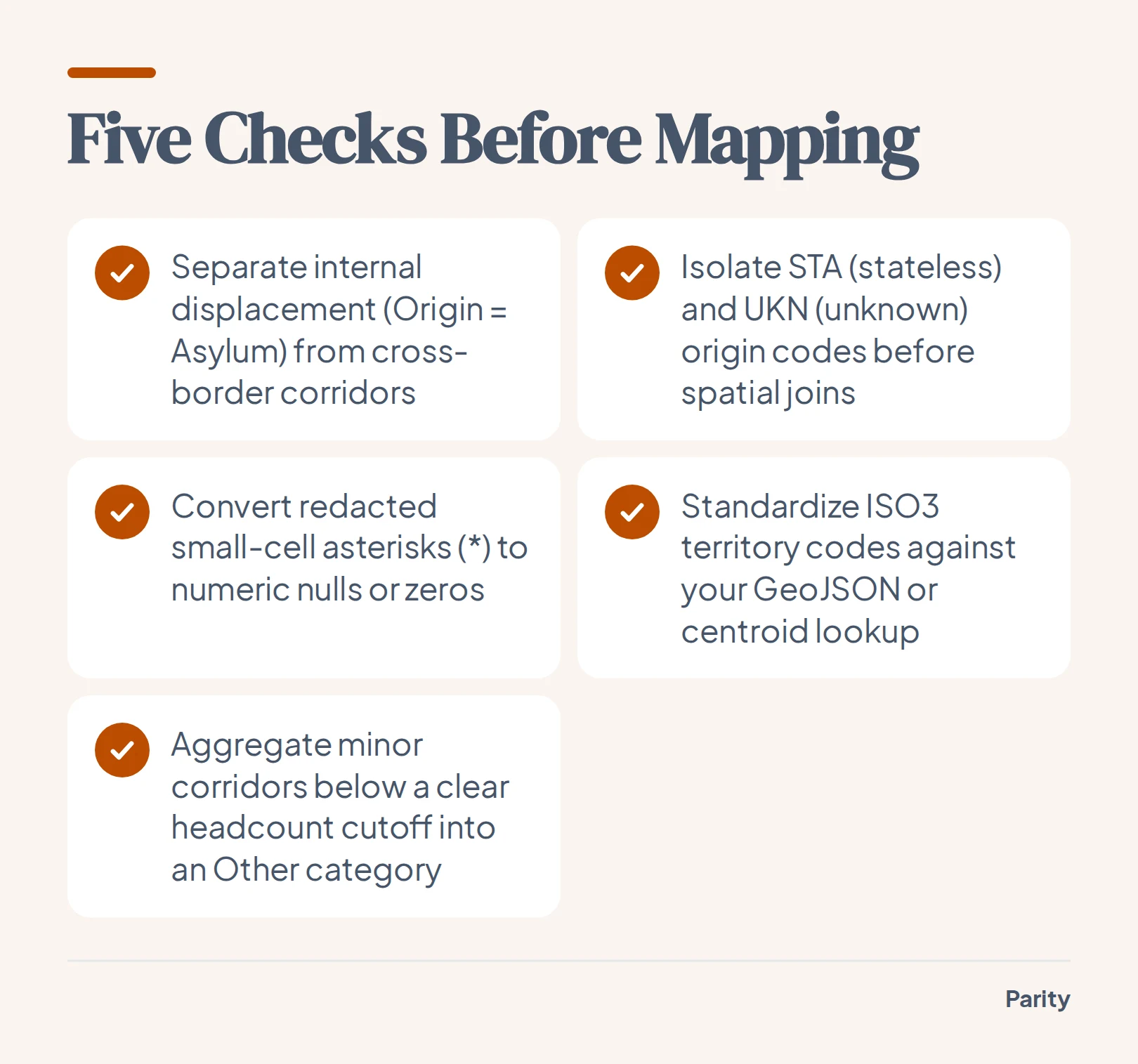
Run through five data hygiene steps before generating a map or network graph:
- Separate internal displacement from bilateral corridors: Filter out rows where the Country of Origin code matches the Country of Asylum code, or where values sit strictly in the IDP column. Mapping internal displacement alongside cross-border corridors distorts bilateral totals.
- Isolate stateless and unknown origin codes: UNHCR tables use special pseudo-ISO codes such as
STAfor stateless persons andUKNorVARfor unknown or various origins. These rows have a valid destination country but no geographic origin polygon, so they must be tallied in a sidebar or footnote rather than dropped. - Handle statistical redaction and small cells: To protect individual privacy in small corridors, public exports often replace counts between 1 and 4 with an asterisk (
*) or round values to the nearest multiple. Convert asterisks to nulls or zero before casting columns to integers, and document the redaction rule in your chart notes. - Align ISO3 codes with your base map: Verify territorial codes (such as Kosovo, Western Sahara, or Tibetan populations) against your polygon lookup table so every reported group maps to a known centroid.
- Set a minimum corridor threshold: A global table contains thousands of tiny bilateral pairs representing fewer than a hundred people. Group corridors below a clear cutoff into an "Other origins" or "Other destinations" bucket so your visual remains legible.
Choosing the right visual for a global refugee migration flow map
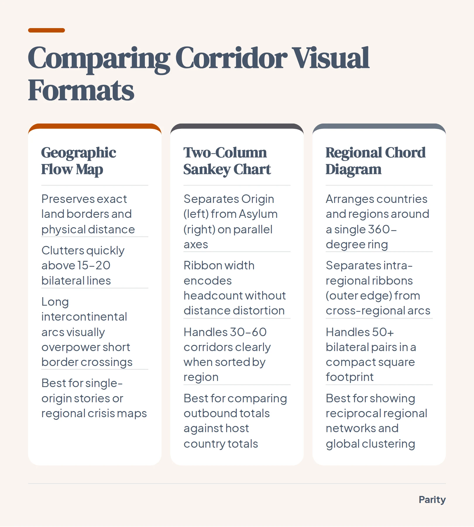
Once your bilateral table is clean, you have to choose how to put it on the page. Drawing curved Bezier lines between country centroids on a world map works only when you show a handful of major routes or filter down to a single origin country.
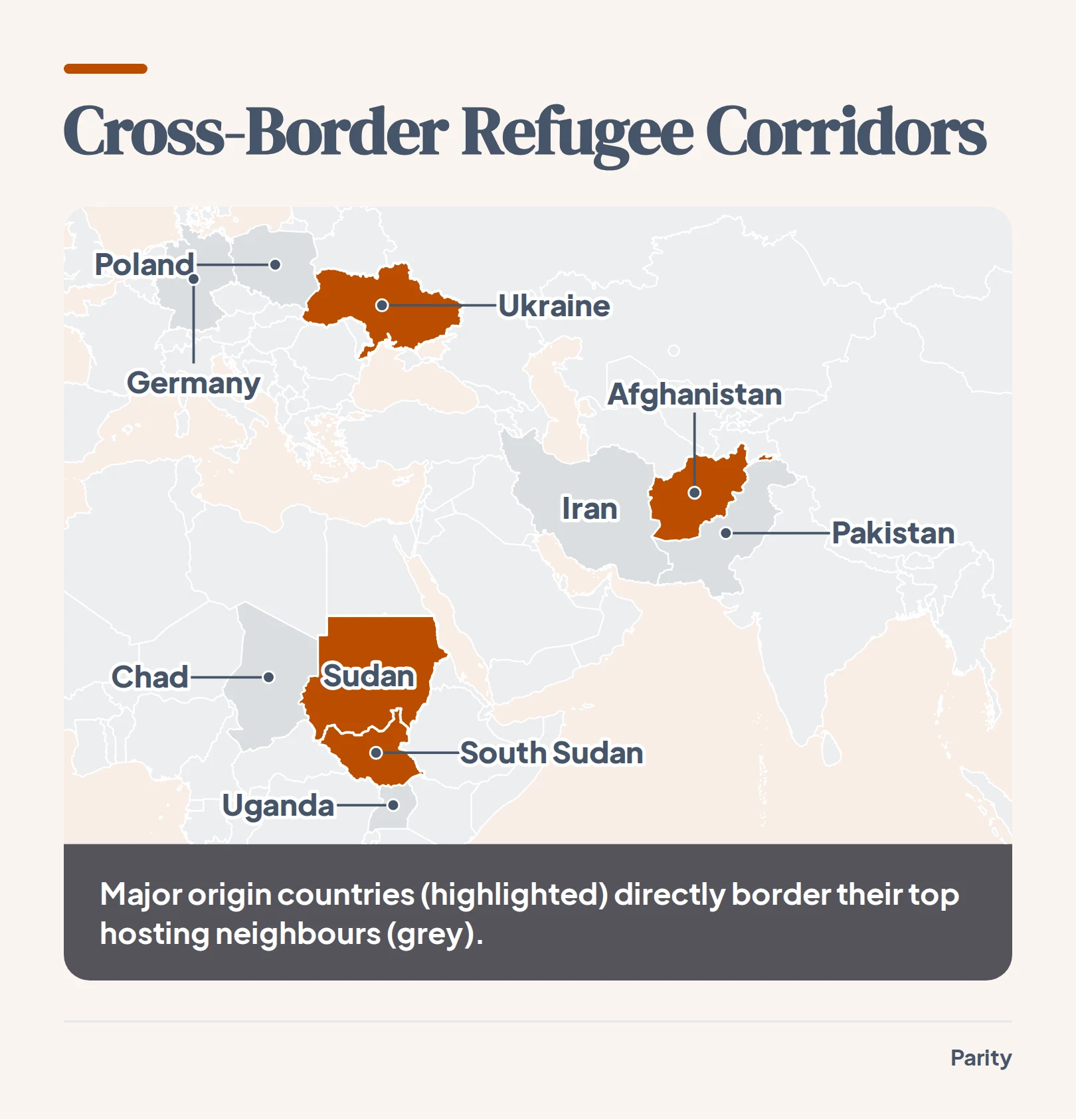
When you plot fifty or more bilateral corridors across the globe simultaneously, long lines crossing oceans dominate the reader's eye even if those corridors carry relatively few people. Meanwhile, the largest displacement movements in the world happen across shared land borders, where short connecting lines turn into illegible knots.
To keep geographic context without creating spaghetti clutter, match the map encoding to the question your reader is asking:
- Proportional symbol maps: Place scaled circles or hex bins at origin and asylum centroids to compare total headcount hosted or displaced without letting large country boundaries distort the visual weight.
- Small multiples by origin: Break a single crowded world map into a grid of regional maps, each showing the outbound corridors from one major crisis country.
- Bilateral matrix or regional grouping: Color countries by region and summarize cross-border totals in sidebars, showing how proximity drives the majority of international protection.
How chord diagrams and Sankey charts show bilateral corridors without map clutter
When the exact volume and pairing of origin-to-asylum corridors matter more than exact latitude and longitude, dropping the geographic base map solves the occlusion problem. Two non-spatial network layouts handle dense bilateral tables cleanly: two-column Sankey diagrams (or alluvial charts) and circular chord diagrams.
A two-column Sankey places countries of origin on the left axis and countries of asylum on the right. Ribbon width is strictly proportional to the number of displaced people in that corridor. A reader can immediately compare total outbound displacement on the left against total hosting responsibility on the right, while tracing exactly how each origin splits across destinations.
A chord diagram arranges countries or world regions around a single circle, sorted by geographic region. Arcs crossing the center connect origins to destinations, while bands hugging the outer rim show movements that stay within the same region, an encoding often used across open-data graphics and global migration chord diagrams.
- Sort nodes by world region: Keep neighboring countries adjacent on the axis or circle so intra-regional movements stay grouped together rather than crossing the entire chart.
- Use directional color encoding: Color ribbons by the origin region so the reader can tell which way a corridor flows at a glance.
- Provide interactive filtering on hover: Let readers highlight a single country node to dim unrelated ribbons and inspect exact bilateral counts.
Historical boundaries, census gaps, and what the bars leave out
Even the cleanest network diagram or proportional map is only as reliable as the administrative registers and surveys behind it. When you plot multi-decade demographic series, sudden jumps or drops in a line often reflect changes in legal definitions or boundary reconstructions rather than physical movement across a border.
This methodological boundary effect appears across many long-term demographic records.
Similarly, historical migration records, whether tracking urban boundary reclassifications or the forced displacement of scientists in the 1930s, require clear methodological notes so readers do not confuse a classification change with an overnight demographic shift. When publishing a graphic from public humanitarian tables, always include three disclosures:
- Cut-off dates and vintage: State whether the data reflect mid-year estimates or end-of-year finalized figures, as emergency movements can shift totals by hundreds of thousands within weeks.
- Included legal categories: Specify exactly which columns you summed (for example, whether asylum-seekers and other people in need of international protection are combined with recognized refugees).
- Registration vs. estimation: Note where host countries rely on individual biometric registration versus government estimates or household surveys.
Building checked dashboards and reports from your own spreadsheets
Turning a multi-thousand-row CSV into a clean chart requires careful aggregation, category filtering, and row-level verification. Whether you are analyzing public demographic tables or internal operational exports, manual pivot tables make it easy to double-count sub-totals or drop unmapped rows.
When you connect a spreadsheet or your business tools to Parity, its AI dashboard generator and AI report generator build interactive charts and written summaries in plain English while operating in read-only mode. Parity checks every calculated number against raw source data, allows you to click any headline number to inspect the underlying query and counted rows, and exports presentation-ready PDF reports with a single click.
Connect a spreadsheet or the tools you run on, and Parity builds the dashboard and writes the report, with every number checked. Try Parity free