How do you map US county migration and multi-decade demographic shifts without area bias?
An analyst opens a spreadsheet of county population estimates and shades every polygon by raw net migration. The resulting map highlights vast rural tracts in the American West while tiny, dense urban counties on the East Coast almost vanish. Just as building an honest sales map by state requires dividing order volume by population, demographic mapping requires encodings that separate land area from human headcount.
When you design maps for regional population growth or domestic migration gains and losses, your first decision is whether to show rates or totals. Choropleth shading works well for per-capita rates or percentage shifts on a diverging color scale. Scaled symbols placed at county centroids better represent raw headcount changes without letting large geographic boundaries dominate the visual field.
At the global level, mapping movement requires separating cumulative stocks from annual flows. According to the UN's International Migrant Stock 2024 and the IOM's Migration Data Portal, 304.0 million people lived outside their birth country by mid-2024, up 98% from 153.9 million in 1990 while remaining under 4% of humanity (about 3.7%).
On the 2024 global migration chord diagram, the circle is split into ten world regions where ribbon width shows migrant numbers: 44% live in another country within their home region, and the largest corridor runs from Mexico to the United States at 11.3 million people.
Stocks versus flows across world regions
A migrant stock counts everyone living outside their country of birth at a specific point in time, blending recent arrivals with people who moved fifty years ago. Comparing UN regional totals between 1990 and 2024 (including migrants of unknown origin) reveals how destination patterns have concentrated:
- Northern America: More than doubled its migrant population from 27.5 million in 1990 to 61.2 million in 2024.
- Europe: Increased from 51.5 million migrants in 1990 to 94.1 million in 2024.
- Sub-Saharan Africa: Rose from 13.8 million in 1990 to 24.3 million in 2024.
- Eastern Asia: Grew from a low base of 4.1 million to 11.6 million as South Korea, Japan, and Hong Kong attracted more foreign workers.
- Central and Southern Asia: Declined from 25.5 million to 20.4 million as Afghan refugees in Iran and Pakistan and former Soviet citizens in Central Asian republics returned, moved on, or died.
When analysts switch from spatial corridors to age structure using population pyramids, another set of encoding rules applies. UN population pyramids are estimates built from censuses, surveys, and vital registration, expressing every bar as a share of the population rather than a raw headcount.
Because countries are reconstructed within present borders, 1975 pyramids for Germany, Russia, and Ukraine reflect modern territories rather than the states of that era, and an open-ended 80+ bar naturally widens as longevity rises.
| Visual encoding | Primary metric | What it reveals | What it hides |
|---|---|---|---|
| Diverging choropleth map | Net migration rate | Regional growth or loss clusters | Total headcount in dense counties |
| Scaled centroid symbols | Raw population change | Absolute gains and losses by place | Exact county boundary shapes |
| Regional chord diagram | Migrant stock corridors | Cumulative origin and destination links | Annual inflows and return moves |
| Population pyramid | Age-sex percentage shares | Demographic momentum and aging | Absolute population size changes |
What does 1,200 years of Kyoto cherry blossom data reveal about long-term climate baselines?
Thermometer networks rarely extend back before the nineteenth century, which limits how far modern warming charts can look into the past. The 1,200-year Kyoto cherry blossom record from 812 to 2026 solves this baseline problem by gathering peak bloom notes from courtier diaries, temple chronicles, poetry, and modern newspapers.
Assembled by climatologist Yasuyuki Aono, published by Our World in Data, and continued from 2026 by Genki Katata, it provides a pre-industrial benchmark spanning more than a millennium.
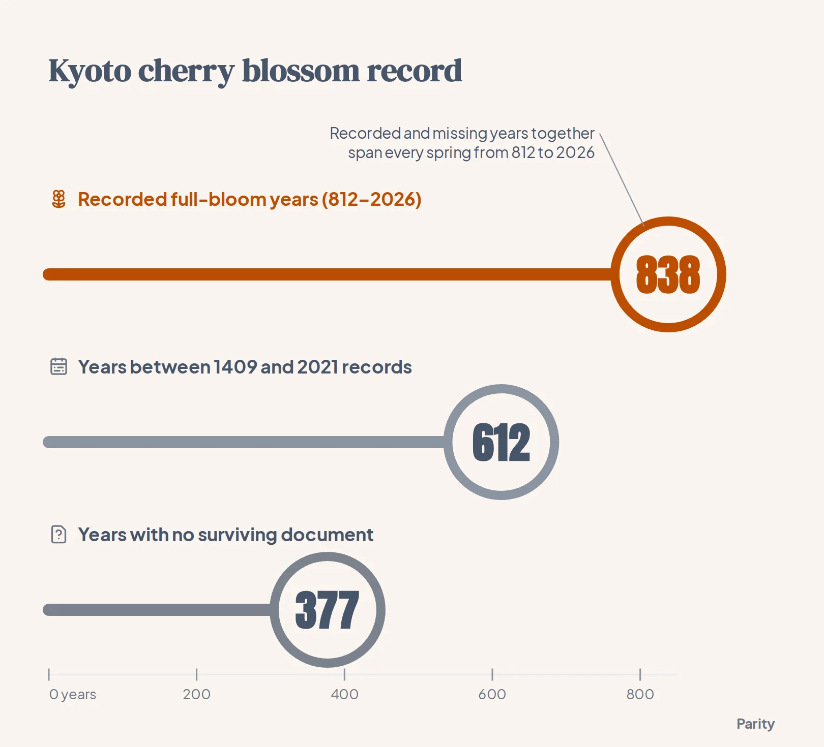
Across the span from 812 to 2026, the dataset contains 838 years with a known full-bloom date and 377 blank years where no historical document survives.
On the visual plate, each spring is plotted by day of the year (higher for earlier blooms, with deeper pink shading) and linked by a brown branch showing the 30-year trailing average. That trailing mean is drawn only when at least ten years inside the 30-year window have surviving records.
Separating urban heat from global climate shifts
In 2021, Kyoto's cherry trees hit full bloom on March 26, breaking a record from 1409 that had stood for 612 years. Research led by Nikolaos Christidis at the UK Met Office alongside Aono and Peter Stott found that human influence shifted Kyoto's flowering roughly 11 days earlier and made an early spring like 2021 about 15 times more likely. Roughly half of that 11-day advance comes from local urban warming as Kyoto expanded, while the remainder reflects broader climate change.
Parallel records in North America show a similar trend over a shorter window. Around the Tidal Basin in Washington, DC, where the National Park Service has monitored Yoshino cherry trees for roughly a century, the Environmental Protection Agency reports that peak bloom has advanced by about eight days since 1921. Washington's earliest recorded peak occurred on March 15, 1990, and in 2026 the trees reached peak bloom on March 26.
How do you plot 73,458 US tornado tracks since 1950 on a single interactive map?
Plotting tens of thousands of overlapping weather events on a single canvas quickly turns into an unreadable blob unless visual weight is tied to severity. In the interactive map of 73,458 US tornado tracks from 1950 through 2025, built from NOAA's Storm Prediction Center database, every storm recorded by the US National Weather Service is drawn as a line from touchdown to lift-off.
Weak storms appear as faint violet threads while the fiercest tracks glow thick and almost white, revealing dense knots across the Deep South and southern Plains and an almost blank region west of the Rockies.
Encoding opacity and stroke width by intensity works because the historical distribution is heavily skewed toward weak events:
- EF0 tornadoes (34,875 tracks): The weakest category, with winds that peel shingles and snap branches.
- EF1 tornadoes (25,179 tracks): Combined with EF0 events, these make up more than four in five recorded tornadoes.
- EF3 to EF5 tornadoes (4.5% of total): The violent end of the scale includes 2,669 EF3s, 596 EF4s, and 60 EF5s (winds above 200 mph), which account for most tornado deaths.
- Longest single track (235 miles): Crossed Louisiana on March 22, 1953, whereas most tracks span just a mile or two.
Scaling extreme weather costs on a seismograph trace
When analysts move from storm paths to financial damage, linear axes often fail because extreme hurricanes dwarf smaller events. On May 8, 2025, NOAA announced that its billion-dollar weather and climate disasters database (covering 1980 through 2024) would be retired with no updates beyond calendar year 2024. Across seven disaster types, that finished record logs 403 events totaling $2.92 trillion in inflation-adjusted 2024 dollars and 16,941 deaths.
To keep smaller events visible alongside major catastrophes, the seismograph chart scales each spike's height by the square root of its cost. Under square-root scaling, a $100 billion hurricane produces a jolt ten times taller than a $1 billion hailstorm rather than a hundred times taller.
For teams building their own weather trackers, our guide on how to analyze climate data dashboards for NOAA weather walks through structuring raw meteorological feeds.
How are global CO2 emissions and daily temperature records structured for visual comparison?
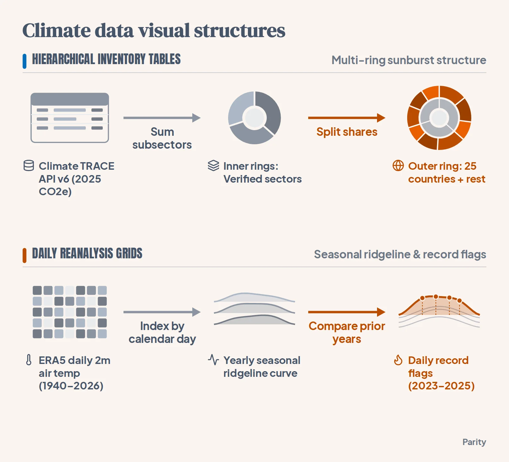
Global climate inventories typically arrive either as nested categorical hierarchies or as dense daily time series. In the 2025 global emissions sunburst by sector and country, data from the Climate TRACE emissions inventory API (version 6) are organized in CO2 equivalent using 100-year global warming potentials.
The inner rings sum subsector activities into verified sector totals (keeping forestry and land use separate), while the outer ring breaks each subsector down across 25 major emitting countries and groups all remaining nations under "rest", with per-second rates calculated across the seconds in 2025.
When tracking resulting temperatures from 1940 to 2026 using ERA5 reanalysis data from the Copernicus Climate Change Service (via Climate Reanalyzer), a stacked ridgeline plot separates seasonal geography from long-term warming. Comparing 1940–1969 with 1996–2025 shows the entire seasonal curve lifting:
- January warming (+0.78°C): The planet's coolest month rose from an average of 11.77°C in 1940–1969 to 12.56°C in 1996–2025.
- July warming (+0.71°C): The warmest month climbed from 15.65°C to 16.35°C over the same multi-decade comparison.
- Top three warmest years: At the bottom of the ridgeline chart, 2024 ranks first (15.09°C annual average, 197 daily records), 2023 second (14.98°C, 208 daily records), and 2025 third (14.97°C).
- Peak daily heat and 1.5°C threshold: Global daily mean temperature peaked in July 2024 (17.15°C on July 23 per Climate Reanalyzer; 17.16°C on July 22 per Copernicus), and 2023–2025 averaged over 1.5°C above pre-industrial levels per Copernicus (1.48°C across eight datasets per WMO, with 2025 at 1.47°C per Copernicus).
What data cleaning steps prevent misleading historical maps and climate charts?
Raw historical tables contain structural quirks that distort charts if plotted without cleaning. Before rendering a multi-decade map or time series, analysts standardize four recurring data edge cases:
- Preserve true missing years and leap-year offsets: In the Kyoto cherry blossom series, blank years mean no document survived rather than a failed spring, and day-of-year figures are mapped to a non-leap calendar where leap years can shift by one day.
- Harmonize scale transitions and segmented paths: Tornadoes before February 2007 used the original Fujita scale before switching to the Enhanced Fujita scale, while straight-line paths omit track width and split state-line crossings into separate database segments.
- Document cross-country definition differences: In the World Bank's 1960–2025 urbanization series (from UN World Urbanization Prospects), each national statistics office defines "urban" differently, and economies under 1 million people are omitted from the stamp sheet for readability.
- Account for reanalysis grid smoothing: When mapping daily 2-metre temperatures across cities using Open-Meteo and ERA5 reanalysis, each grid cell averages several kilometres across city and countryside, which can understate urban heat islands and differ by a degree or two from station gauges.
Watch out: Never interpolate zeros across missing historical observations. Filling Kyoto's 377 undocumented springs with placeholder numbers would corrupt the 30-year trailing average, which is why the branch line only renders when at least ten years in a window have records.
How can you build interactive dashboards from your own spreadsheets and verify every number?
Turning raw tables into verified visuals does not require writing custom rendering scripts from scratch. When you connect a spreadsheet or link your business tools, Parity's AI dashboard generator and AI report generator build interactive dashboards and written reports in seconds or minutes.
Instead of relying on partial data samples, Parity analyzes complete datasets and verifies every number against the underlying rows. You can use plain-English prompts in the chat interface to customize chart layouts and breakdowns, and Parity also tells you what to look at next:
- Read-only connectors for 54 tools: Connect spreadsheets, accounting software, online stores, ad platforms, and social accounts without ever altering your source data.
- Clickable Data Audit: Click any headline figure on your dashboard to inspect the underlying query and counted rows.
- Flexible deployment and export: Run on Cloud Hosted infrastructure or a Local Mac Mini (a lower maintenance tier that keeps full data sovereignty on office hardware), and export presentation-ready PDF reports in one click.
Connect a spreadsheet or any of 54 supported tools to build an interactive dashboard and written report in seconds. Try Parity free