What you need
Pulling a 75-year weather CSV from a public server takes thirty seconds. Turning that file into a chart that does not mislead your readers takes a careful workflow. An uncleaned storm database will show a dramatic rise in weak tornadoes since 1950 that is actually the invention of Doppler radar and storm-spotter networks.
Whether you are an operations team pricing regional weather risk, a researcher tracking temperature anomalies, or a journalist charting storm damage, the steps are the same. You have to separate instrument changes from physical trends before you plot a single line. Before starting the first step, gather these four essentials:
- A raw public climate file: Download a structured file in CSV, Excel (.xlsx), or .xls format, such as the Storm Prediction Center file
1950-2025_actual_tornadoes.csvor the HURDAT2 best-track release. - Dataset documentation: Keep the agency's methodology notes open so you know when rating scales changed, how missing values are coded, and which baseline years define the normal average.
- A boundary or grid reference: If you are mapping tracks or city temperatures, note whether your records use US Census Bureau state boundaries or a model grid cell several kilometres across.
- An AI dashboard generator: Use a workspace like the Parity AI dashboard generator to profile every row, build your initial interactive dashboard, and verify summary metrics against the source file.
1. Pick the right NOAA dataset for your question
Climate and weather analysis fails when you ask a dataset to answer a question it was never designed to measure. Across the 55 public-data stories and 85,763 words published on Parity's data desk, including the U.S. billion-dollar disasters seismograph (1980–2024), matching the question to the instrument record is always the first decision.
Public agencies publish both direct station observations, which record local weather at a single point, and gridded reanalysis datasets, which blend billions of observations from satellites, balloons, ships, and stations into a global weather model. You can download station and regional summaries from NOAA's National Centers for Environmental Information, or pull hazard-specific files for severe storms and tropical cyclones.
Match your question to the instrument record
- Financial disaster losses: The NOAA NCEI U.S. Billion-Dollar Weather and Climate Disasters record covers 1980–2024 and counts 403 events totaling $2.92 trillion in CPI-adjusted 2024 dollars and 16,941 deaths.
- Dataset handoffs: On May 8, 2025, NOAA announced the billion-dollar disaster database would be retired "with no updates beyond calendar year 2024"; project lead Adam Smith left the agency in April 2025 for Climate Central, which restarted the tally later in 2025 and recorded 14 events costing over $101 billion in the first half of 2025.
- Local severe weather tracks: In our analysis of every U.S. tornado from 1950 to 2025, the official Storm Prediction Center record holds 73,458 tornadoes mapped from touchdown to lift-off.
- Tropical cyclone intensity: In our Atlantic hurricanes radar analysis, the National Hurricane Center's HURDAT2 file tracks post-season positions from 1851–2025 every six hours with maximum sustained winds in knots, Saffir-Simpson categories (where Category 5 is 137 knots or more), and Accumulated Cyclone Energy (ACE) in units of 10⁴ kt².
| Dataset | Time Span | Primary Metrics | Key Caveat |
|---|---|---|---|
| NCEI Billion-Dollar Disasters | 1980–2024 | 403 events, CPI-adjusted 2024 $ | Retired by NOAA after 2024; revived by Climate Central |
| SPC Tornado Database | 1950–2025 | 73,458 tracks, F and EF ratings | 1950s weak tornado counts underreported before Doppler radar |
| NHC HURDAT2 Hurricanes | 1851–2025 | Wind in knots, ACE in 10⁴ kt² | Uses 1991–2020 for long-term averages |
| ERA5 Reanalysis | 1940–2026 | Hourly and daily 2 m air temperature | Grid cells smooth local urban and terrain extremes |
2. Clean historical quirks and scale changes before charting
Once you download your CSV, inspect the columns for sentinel values, rating transitions, and spatial averaging before you build any summary tables. If you sum or average raw climate columns without checking how the data were logged across decades, your charts will display artifacts of data collection rather than weather.
In the NOAA Storm Prediction Center tornado file (1950-2025_actual_tornadoes.csv), four cleanup rules keep the historical comparison honest:
- Harmonize rating scale cutoffs: Tornadoes are rated on the original Fujita scale before February 2007 and on the Enhanced Fujita scale since then, so align your category labels across that date.
- Recode sentinel missing values: Tornadoes with an unknown rating are coded as −9 in the database; recode −9 as EF0 (or filter them into an unrated bucket) so a −9 integer never drags down numerical averages.
- Check multi-state track deduplication: Verify whether tracks crossing state borders appear once or per state; in
1950-2025_actual_tornadoes.csv, cross-border tracks are stored once. - Separate early observational eras: Because weak tornadoes frequently went unreported in the 1950s before Doppler radar and spotter networks, filter trend charts to stronger tornadoes or modern radar decades.
Temperature grids need similar care. When pulling daily 2 m maximum, minimum, and mean air temperatures from the Copernicus ERA5 reanalysis (via the Open-Meteo Historical Weather API or Climate Reanalyzer), remember that each value represents a grid cell several kilometres across. The grid averages city and countryside, park and pavement.
Urban areas experience elevated temperatures compared to outlying rural areas because buildings and pavement absorb and re-emit heat.
Watch out: When comparing an incomplete current year against historical records, filter every earlier year to the exact same calendar days before averaging so seasonal cycles do not skew the rank.
3. Separate weather noise from long-term climate and exposure trends
A single hot summer or quiet hurricane season tells you about the weather; decades of records tell you about the climate. In a multi-decade grid of Arctic sea ice across September minimums, reading across a single row shows year-to-year noise (1996 is larger than its neighbors, while 2012 is far smaller), whereas reading down the columns reveals the steady decade-over-decade shrinking.
When analyzing financial disaster records, you must also separate physical weather from human exposure. NOAA's billion-dollar disasters table adjusts losses to 2024 dollars using the Consumer Price Index, which accounts for inflation but not for population growth or wealth accumulation in hazard zones like the Gulf Coast, Florida, the suburbs of Dallas, or the hills around Los Angeles.
- Control for exposure and vulnerability: Note in your dashboard commentary that Climate Central attributes rising disaster tallies both to climate change and to increased exposure and vulnerability, or "where we build; how we build".
- Acknowledge methodological debate: Political scientist Roger Pielke Jr. has argued that the billion-dollar tabulation does not meet NOAA's information quality standards for detecting extreme weather trends, while defenders note the dataset was built to count direct economic costs rather than isolate climate change.
- Track ocean-atmosphere cycles: Overlay global temperature trends with Pacific phases; NOAA's Climate Prediction Center tracks El Niño, which releases ocean heat into the atmosphere with a lag of a few months and contributed to the record heat of 2023 and 2024.
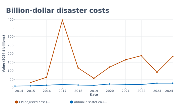
In the NCEI annual series from 2014 to 2024, annual event counts climbed from 10 disasters in 2014 and 11 in 2015 ($30.9 billion) to 27 events in both 2023 ($90.5 billion) and 2024 ($183 billion, 568 deaths), while CPI-adjusted damage peaked in 2017 at $396 billion across 19 events and 3,280 deaths.
4. Choose chart encodings that handle extreme spikes
Weather datasets are heavily skewed. Most tornadoes are weak, most days sit near the seasonal norm, and a single hurricane season can cause 10 × the damage of a quiet year. Standard linear bar charts and opaque map pins turn these distributions into unreadable walls of ink.
When we designed the global temperature ridgeline (1940–2026) and our storm maps, we chose encodings that preserve both everyday baselines and extreme outliers:
- Overlapping ridgelines for daily temperatures: Stack 87 yearly lines (1940 at the top to 2026 at the bottom) from January to December and shade years below the 1991–2020 norm in white and warmer years from orange to red; through October 2, 2026, the 2026 ridge averaged 15.30°C (behind 2024 at 15.38°C over the same days, ahead of 2025 at 15.26°C and 2023 at 15.20°C) and peaked at 17.05°C on August 14, 2026.
- Squared-wind energy metrics for cyclones: Instead of counting named storms alone, chart Accumulated Cyclone Energy (ACE), which sums the square of maximum sustained wind (in units of 10⁴ kt²) at each six-hourly fix against the 1991–2020 average.
5. Use AI to analyze data and build an interactive dashboard
Once you understand your dataset's structure and caveats, you do not need to spend hours wrestling with spreadsheet chart wizards or writing code. Deciding what questions your dashboard should answer comes first; then Parity AI handles the layout in seconds without formulas or manual data modeling.
Follow these steps to turn your cleaned NOAA export into an interactive dashboard and a client-ready report:
- Upload your spreadsheet: Drop your CSV,
.xlsx, or.xlsfile into Parity over an encrypted connection; Parity reads every row (not a sample), profiles the columns, and never uses your file to train models. - Generate the initial view: Describe what you want to see in plain English, and Parity AI builds an interactive dashboard complete with charts, KPI cards, tables, and written insights.
- Refine charts by chatting: Prompt Parity in plain English to group tornado counts by Enhanced Fujita rating, filter out pre-2007 Fujita rows, or compare 2024 disaster costs against 2017, and the dashboard updates in place.
- Export a pixel-perfect PDF: When your analysis is ready for stakeholders, export a pixel-perfect PDF in one click that matches the on-screen layout.
6. Verify every calculated metric against the raw rows
A climate chart is only as credible as the row count behind it. If a stakeholder asks why 2017 shows $396 billion in damage or whether cross-border tornado tracks were counted twice, you need to inspect the exact rows that produced the headline figure.
Parity operates in a read-only manner that never alters your source files or connected tools, and every number is checked against your data before you see it. You can click on any headline number on your dashboard to inspect the underlying queries and raw counted rows.
- Audit category totals: Click a KPI card to confirm that sentinel codes like −9 were excluded from average intensity calculations.
- Verify date filters: Check the query range on partial-year comparisons so an October temperature cut matches the exact calendar day across all historical years.
- Re-run recurring cycles: When the next seasonal or monthly release drops, re-run your report on the new file to keep a consistent layout across reporting cycles.
Upload an Excel or CSV file or connect QuickBooks and Xero to build a verified dashboard in seconds. Try Parity free