To apply conditional formatting based on another cell in Excel, select the cells you want to colour, go to Home › Conditional Formatting › New Rule › Use a formula to determine which cells to format, and type a formula that points at the other cell, such as =$G2="On hold". Write the formula for the first row of your selection, put a $ in front of anything that shouldn't move, and pick a format.
That last sentence is where nearly every broken rule goes wrong. Excel doesn't store one formula per cell. It stores one formula, written for the top-left cell of the range, and slides it across every other cell the way it would slide a formula you copied. Get the sliding right and you can colour a cell, a row or a column from any cell in the workbook. Get it wrong and the shading lands one row low, in one column only, or everywhere.
This guide works through five rules on one sheet. The example business is Dunmore Freight, a fictional regional carrier with twelve consignments in its last week of September. Download the practice workbook (.xlsx) to follow along: the Practice sheet has the data with no rules, and the Solution sheet has all five in place.
How Excel reads a formula rule
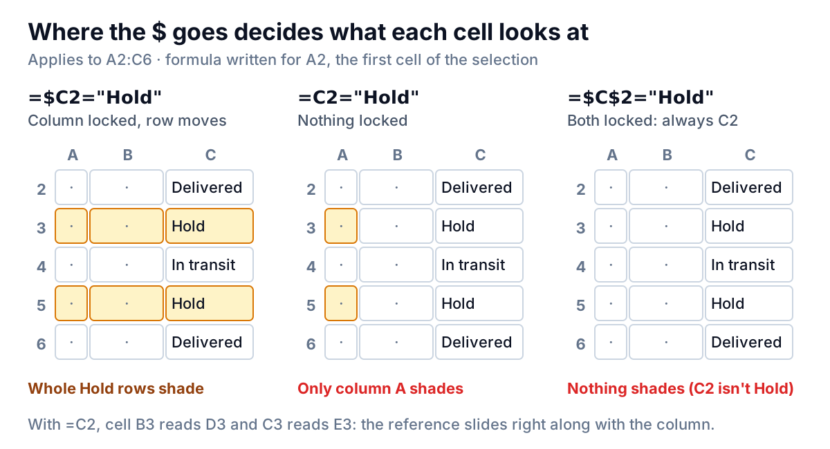
Before the examples, the one idea that makes all of them work. When you select A2:C6 and enter a rule, Excel treats your formula as if it were typed into A2, the active cell. For every other cell, it shifts the references by the same distance, exactly like copying a formula. So the $ signs decide what each cell looks at.
| You write | Column | Row | Use it for |
|---|---|---|---|
$G2 | Locked | Moves | Whole rows: every cell in row 5 reads G5 |
G2 | Moves | Moves | A cell compared with a neighbour in the same row, applied to one column |
$M$2 | Locked | Locked | A single settings cell: a target, a limit, an as-of date |
G$2 | Moves | Locked | Whole columns from a header row, such as shading this month's column |
Microsoft's own instructions make the same point in fewer words: when you click a cell while writing the rule, Excel inserts an absolute reference, and you use relative references if you want Excel to adjust them for each cell. Clicking G2 gives you $G$2, which is almost never what a row rule needs. Press F4 to cycle through $G$2, G$2, $G2 and G2, or just delete the $ you don't want.
Five ways to use conditional formatting based on another cell
Dunmore's sheet has one row per consignment: number, customer, lane, pickup date, promised delivery date (E), delivered date (F, blank until delivered), status (G), weight in kg (H) and charge. Two settings sit beside the data: the as-of date in M1 (30 September 2026) and the heavy-load limit in M2 (1,500 kg). A third sheet, Credit hold, lists customers the office manager has put on hold for unpaid bills.
1. Compare with a neighbour in the same row
Flag deliveries that arrived after the promised date. Select F2:F13 and enter:
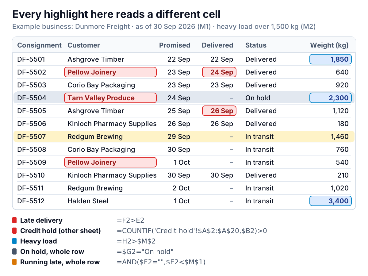
=F2>E2No $ at all, because the rule only covers one column and each cell should compare with the cell to its left. F5 reads E5, F6 reads E6. Two consignments light up: DF-5502 for Pellow Joinery (promised 23 September, delivered the 24th) and DF-5505 for Ashgrove Timber (promised the 25th, delivered the 26th). Blank delivered dates count as zero, which is never later than a date, so undelivered loads stay clear.
2. Compare with one settings cell
Flag loads heavy enough to need the bigger truck. Select H2:H13 and enter:
=H2>$M$2H2 moves down the column; $M$2 stays put. Three loads pass the 1,500 kg limit: 1,850, 2,300 and 3,400 kg. When the new truck arrives and the limit changes, edit M2 and the sheet re-reads itself. If this is the only kind of rule you need, the built-in Highlight Cells Rules › Greater Than does the same job when you click M2 in its box.
3. Shade the whole row from one column
Grey out consignments that are on hold. Select A2:I13, with A2 as the active cell, and enter:
=$G2="On hold"The $ before G keeps every column looking at the status column; the free row number lets row 5 read G5. Text goes in double quotes, and the match isn't case-sensitive, so "on hold" works too. DF-5504 for Tarn Valley Produce turns grey.
4. Combine conditions with AND or OR
Flag loads that are not delivered and already past their promised date. Select A2:I13 and enter:
=AND($F2="",$E2<$M$1)Both halves must be true. DF-5507 for Redgum Brewing, promised on the 29th and still in transit on the 30th, turns amber. DF-5508 was promised on the 30th, the as-of date itself, so < leaves it out; use <= if "due today" should count as late. Swap AND for OR when either condition is enough, for example =OR($G2="On hold",$G2="Damaged").
5. Read a list on another sheet
Flag customers on the Credit hold sheet. Select B2:B13 and enter:
=COUNTIF('Credit hold'!$A$2:$A$20,$B2)>0COUNTIF counts how many times this row's customer appears in the hold list; more than zero means they're on it. The list range is fully locked and leaves room for more names; the customer cell moves with the row. Pellow Joinery (twice) and Tarn Valley Produce are flagged.
A defined name makes this easier to read and maintain. Select the list, type CreditHold in the Name Box left of the formula bar, and the rule becomes =COUNTIF(CreditHold,$B2)>0. When the list grows, you change the name's range once in Formulas › Name Manager.
What you can't do is point the rule at a different file. Microsoft says plainly that you can't use conditional formatting on external references to another workbook. If the hold list lives in the accounts team's file, copy it into a sheet in your workbook, or link a sheet to it with ordinary cell formulas and point the rule at that sheet.
Order the rules: narrow ones first
DF-5504 meets four of the five rules. Its customer is on credit hold, it weighs 2,300 kg, it's on hold, and it's past its promised date with no delivery. When rules set the same thing, such as fill colour, the rule higher in Home › Conditional Formatting › Manage Rules wins; Microsoft documents this as precedence from top to bottom.
The solution workbook puts the single-column rules (late delivery, credit hold, heavy load) above the whole-row rules (on hold, running late). That way DF-5504's customer cell stays red and its weight stays blue inside a grey row. If the row rules came first, their fill would cover every cell in the row and hide the more specific warnings. Between the two row rules, on hold sits above running late, because "on hold" explains why it's late.
Switch Show formatting rules for to This Worksheet to see all five, and use the arrow buttons to reorder them. For more on managing a growing list of rules, including Stop If True and fragmented ranges, see our main guide to conditional formatting in Excel.
Mistakes that make the highlight land in the wrong place
The off-by-one row
This is the most common one. You select A2:C6, but write the rule as if it starts in row 1, so =$C1="Hold". Excel reads that as "the row above", and every highlight lands one row below the row you meant.
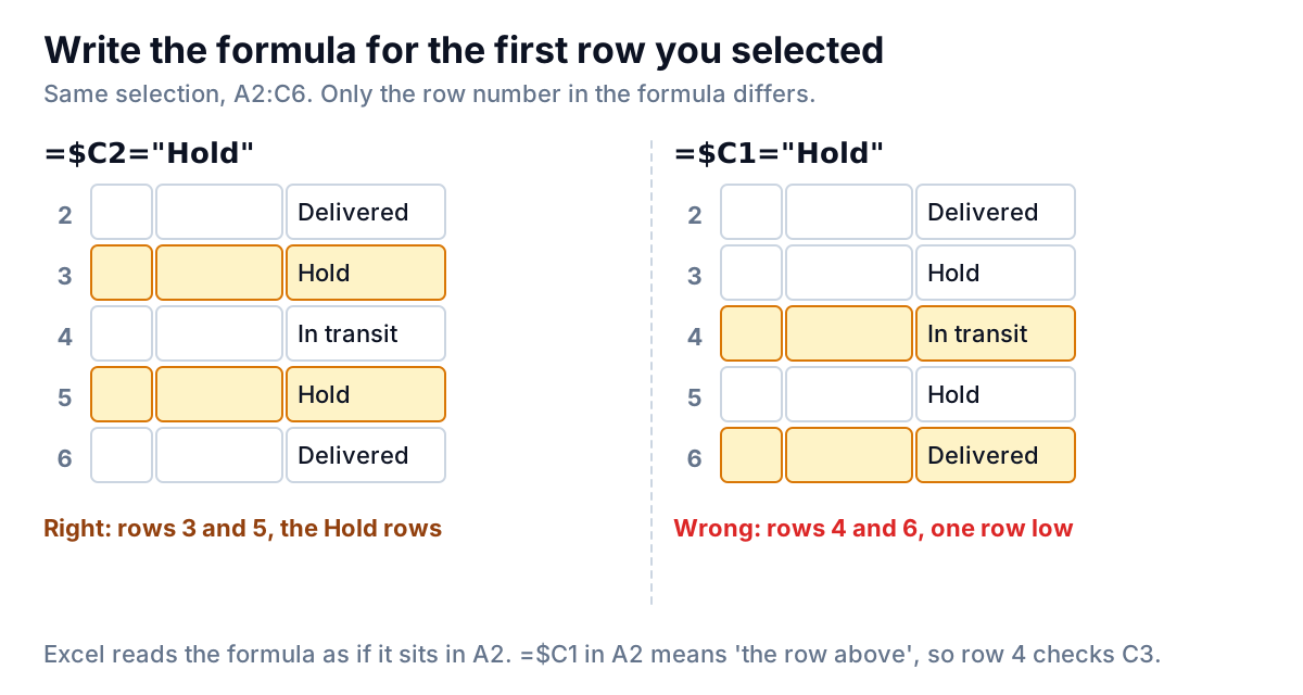
It also happens when you click a column header to select the whole column and then write $G2. The selection starts at row 1, so write $G1 instead, or select from row 2 down.
The rest of the list
| Symptom | Cause | Fix |
|---|---|---|
| Only column A shades | G2 without the column $, so column B reads H, C reads I | $G2 |
| Every row shades, or none | $G$2 from clicking the cell: every row checks row 2 | Remove the $ before the row number |
| Text rule never fires | Missing quotes (=$G2=On hold), or a trailing space in the data ("On hold ") | Quote the text; clean the column with TRIM, or test with =TRIM($G2)="On hold" |
| Rows with a blank date are flagged | A blank cell counts as zero, and zero is earlier than any date | Add a guard: =AND($E2<>"",$F2="",$E2<$M$1) |
| A number rule ignores some rows | Numbers stored as text, common in exports | Convert them with Convert to Number or VALUE |
| Rule shows nothing at all | The formula returns an error, which counts as not true | Test it in a spare column (below) |
Google Sheets works differently
Google Sheets has the same idea under Format › Conditional formatting › Custom formula is, with the same $ logic. The main difference is references to other sheets: Google's help says custom formulas can only reference the same sheet directly, and other sheets through INDIRECT. Our guide to Google Sheets conditional formatting based on another cell covers it step by step.
When the sheet is really a status board
Dunmore's sheet is a status board: what's late, what's stuck, which customer is on hold. Conditional formatting based on another cell handles that well while the list is short and one person maintains it. It gets harder when the data comes out of a transport system every morning as a fresh export, the hold list lives with the accounts team, and someone wants weekly on-time rates by lane as well. Then you're rebuilding the sheet each day and re-checking that the rules still cover the right range. If you're tracking those weekly rates in a spreadsheet, our KPI tracking template gives you a starting layout.
Parity takes that export as a CSV or Excel upload and builds a dashboard from it: headline numbers with their trends, charts, what explains them, and a table of what needs attention, like the consignments past their promised date. Every number is checked against queries on the full dataset before you see it. When tomorrow's export arrives, you update the dashboard with the newer file instead of rebuilding it.
Upload your consignment or job export and get a checked dashboard with late and stuck items listed for you. Build a report from your data free
For a sheet you maintain by hand, though, the five patterns above cover almost every use of conditional formatting based on another cell: a neighbour in the same row, one settings cell, a whole row from one column, AND and OR, and a list on another sheet. Write each formula for the first selected row, lock only what shouldn't move, and test it in a spare column before you trust the colours.