To format cells in Google Sheets based on another cell, select the cells to colour, open Format > Conditional formatting, set "Format cells if…" to Custom formula is, and type a formula that's TRUE when the colour should show, such as =$F2<=2. Write the formula for the first row of your selection, put a $ in front of the column you're checking, and Sheets applies it to every row below.
Google's conditional formatting help page covers the menus. This guide is about the formula, because that's where these rules go wrong: a colour that lands one row off, a rule that only colours one column of a row, or a reference to another tab that Sheets won't accept. We'll build four rules on one tutoring roster, from a single highlighted name to a whole row driven by a list on another sheet.
The example business is Clover Hill Tutoring, a fictional tutoring company. Families prepay for a block of hours, and the office tracks ten students: tutor, subject, hours bought, hours used, hours left, last session date, invoice due date, and a Paid? column. A second tab, "Paused", lists students taking a break. The examples use 7 October 2026 as "today". Download the practice workbook (.xlsx); upload it to Google Drive and open it in Sheets, or use File > Import. The Solution sheet has all four rules applied, plus columns that show each rule as TRUE or FALSE per row. Rules normally come through the import; if one doesn't, the How to use sheet lists each rule to type in, and the checkbox column arrives as TRUE/FALSE until you add tick boxes with Insert > Checkbox.
The idea behind conditional formatting based on another cell
A custom formula rule is a TRUE-or-FALSE question that Sheets asks once for every cell in the "Apply to range" box. If the answer is TRUE, that cell gets the format. The formula you type is the version for the top-left cell of the range. For every other cell, Sheets moves the references by the same distance, exactly as it would if you copied a formula down a column.
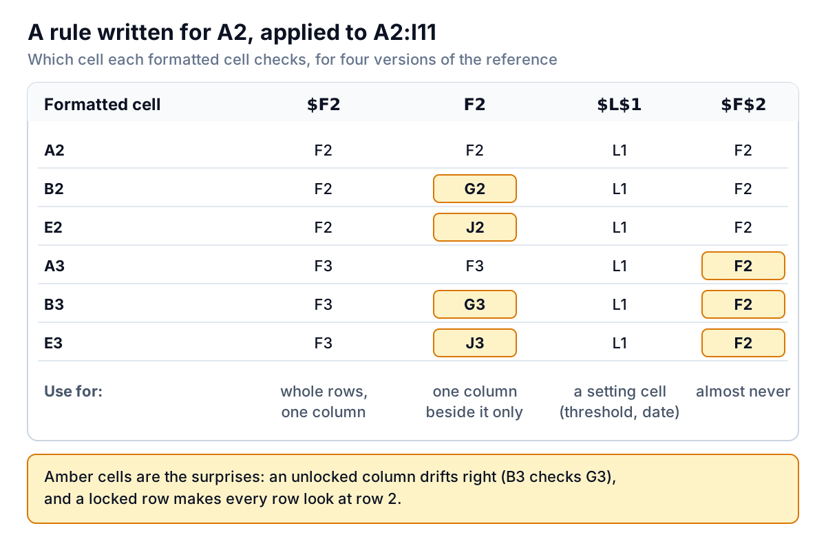
Dollar signs stop that movement. Google's help says you will often need them "so that the formatting is applied using absolute references". In practice there are three versions of a reference, and choosing between them is the whole skill:
$F2: the column is locked, the row moves. Every cell in row 5 looks at F5, whatever column it's in. Use this for whole-row rules and for checking one column from another.$L$1: both are locked. Every cell looks at L1. Use this for a single setting cell, such as a threshold or a date.F2: nothing is locked. A cell in column B looks at G, two columns to the right of where you meant. Use this only when the range is a single column and you want the cell to check its neighbour.
Rule 1: highlight one cell based on another cell
The office wants a student's name to turn amber when their prepaid hours are almost used up, so someone calls the family before the last session. Hours left are in column F (=D2-E2). The alert level goes in a setting cell, L1, set to 2.
- Select A2:A11, the names.
- Click Format > Conditional formatting. The side panel opens with A2:A11 in "Apply to range".
- Under "Format cells if…", choose Custom formula is.
- Type
=$F2<=$L$1. - Pick an amber fill under "Formatting style" and click Done.
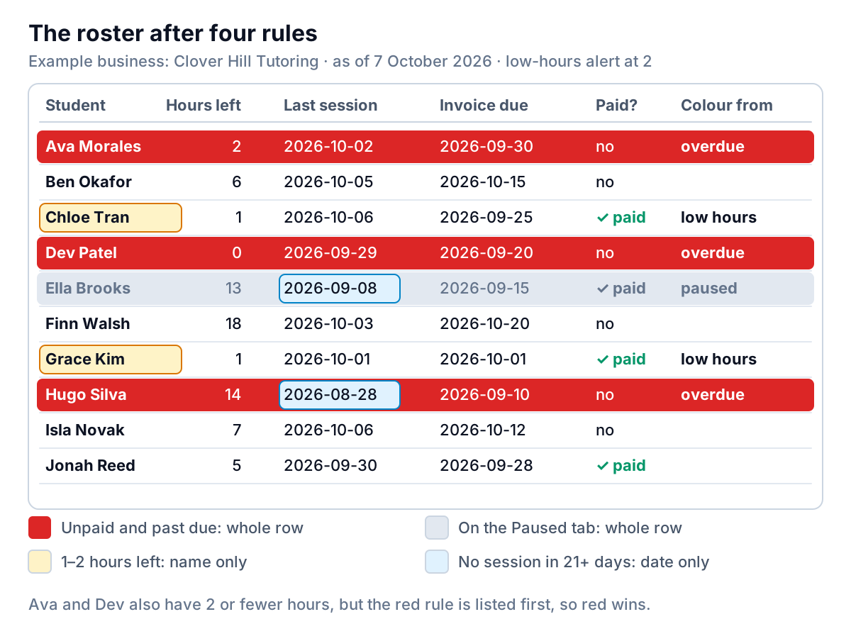
Four names light up: Ava Morales (2 hours left), Chloe Tran (1), Grace Kim (1) and Dev Patel (0). Change L1 to 5 and Jonah Reed (5 left) joins them, without touching the rule. Putting thresholds in a cell rather than inside the formula is the habit that saves you from editing rules every time the business changes its mind.
The formula starts with an equals sign and must return TRUE or FALSE. =$F2<=$L$1 does. =$F2 on its own doesn't really, because any non-zero number counts as TRUE and you'd colour almost everything.
Rule 2: highlight the whole row
An unpaid invoice past its due date should make the whole row red, so it can't be missed while scrolling. The test needs two columns: Paid? in column I (a checkbox, which holds TRUE when ticked and FALSE when not) and the due date in column H. "Today" is in L2.
- Select A2:I11, every column of the roster.
- Format > Conditional formatting > Custom formula is.
- Type
=AND($I2=FALSE, $H2<$L$2). - Choose a red fill with white text, and click Done.
The $ before I and H is what makes it a row rule. Every cell in row 2, from A2 across to I2, checks I2 and H2. Without it, B2 would check J2 and K2 (empty), and only part of the row would turn red. Three rows match: Ava Morales (due 30 September), Dev Patel (due 20 September) and Hugo Silva (due 10 September). Chloe Tran's invoice was due 25 September but is ticked as paid, so her row stays clear.
In a live sheet, replace $L$2 with TODAY(): =AND($I2=FALSE, $H2<TODAY()). The workbook keeps a fixed date in L2 so the colours match this article; type =TODAY() into L2 and the rule becomes live without editing it.
=$I2<>"Yes".Rule 3: format based on a cell in another sheet
Students on a break are listed on the "Paused" tab: Ella Brooks (exam leave), Hugo Silva (travelling) and a former student, Maya Lin. The office wants their rows greyed out on the main roster.
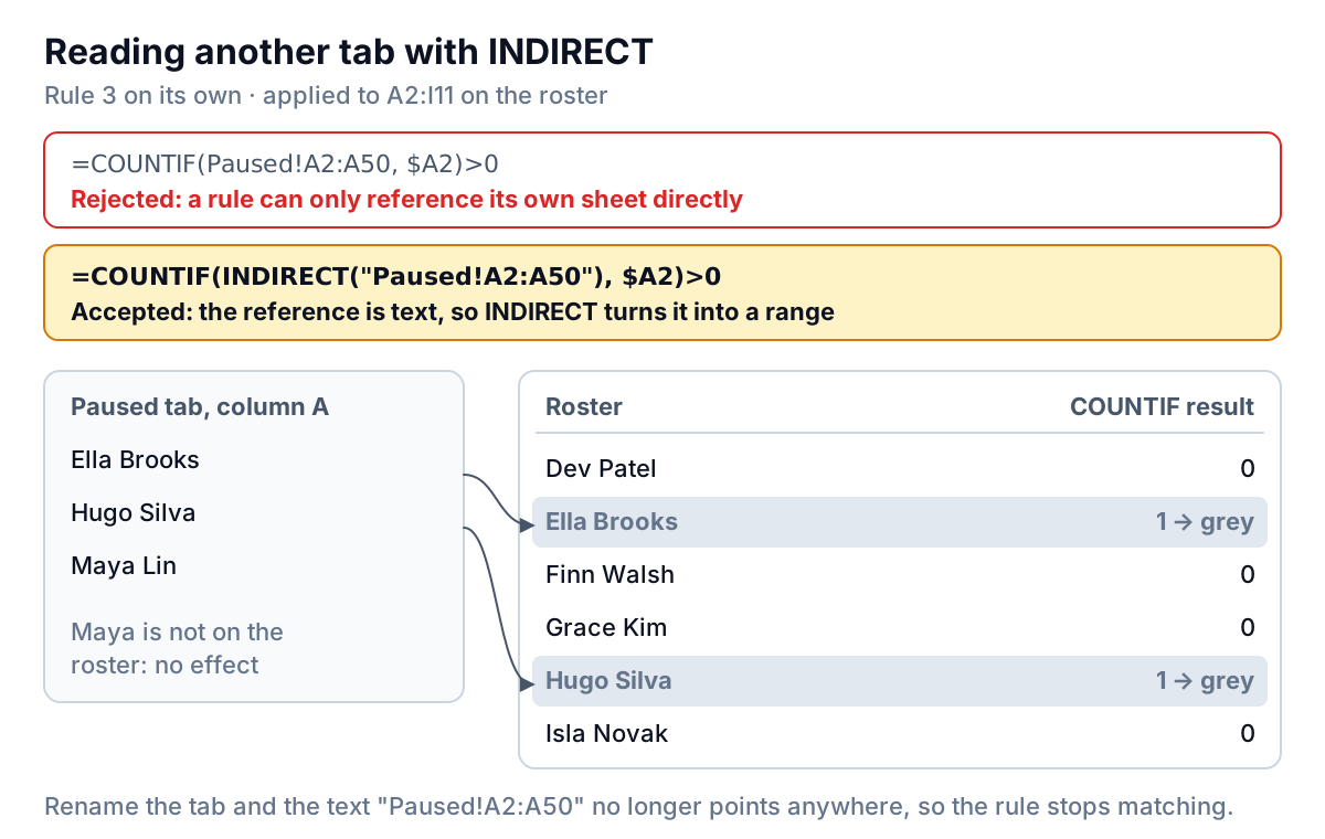
The obvious formula, =COUNTIF(Paused!A2:A50, $A2)>0, is refused. Google's help is explicit: custom formulas can only reference the same sheet directly, and "to reference another sheet in the formula, use the INDIRECT function". INDIRECT takes a reference written as text and turns it into a real one, which gets around the restriction:
=COUNTIF(INDIRECT("Paused!A2:A50"), $A2)>0Apply it to A2:I11 with a grey fill and grey text. COUNTIF counts how many times the student's name appears on the Paused list; anything above zero means paused. Ella's and Hugo's rows turn grey. Maya Lin isn't on the roster, so she has no effect.
Three details make INDIRECT rules behave:
- The reference is text, so it never adjusts. If someone renames the tab to "On break", the rule silently stops matching. If you insert a column on the Paused tab, it keeps reading column A. Keep those tabs boring and stable.
- Quote tab names with spaces. A tab called "Paused students" needs single quotes inside the double quotes:
INDIRECT("'Paused students'!A2:A50"). - Give the list room to grow. A2:A50 covers far more than three names, and blank cells don't count. An open-ended "Paused!A2:A" also works.
The same pattern handles lookups. To highlight hours used above a family's agreed cap kept on a "Packages" tab, you'd compare against VLOOKUP($A2, INDIRECT("Packages!A2:B50"), 2, FALSE); our guide to VLOOKUP in Google Sheets covers the lookup itself.
Rule order: when two rules want the same cell
Hugo Silva is both paused and overdue. Ava Morales is both overdue and low on hours. Which colour wins? Google's answer: "Rules are evaluated in the order listed. The first rule found to be true will define the format of the cell or range." Each cell takes the format of the first rule in the list that's true for it.
For Clover Hill, the rules are listed in this order:
- Last session more than 21 days ago, date cell light blue:
=$L$2-$G2>21on G2:G11. - Overdue and unpaid, whole row red.
- Paused, whole row grey.
- Low hours, name amber.
The date rule goes first because it only touches one column, so it can't hide anything else, and it would otherwise disappear under the row colours. After that, money comes first. Hugo's row is red, not grey, because someone still needs to chase his invoice, and his last-session date (28 August, 40 days earlier) shows light blue inside the red. Ava's and Dev's names are red rather than amber, which is right: the overdue invoice is the bigger problem. Ella's row is grey, with her last-session date (8 September, 29 days earlier) in light blue. To change the order, drag a rule up or down in the side panel by the handle on its left.
Notice what the order did to Rule 1: two of its four amber names are now red. That's a choice, not a bug. Decide what matters most for each cell and list it first; that decision is the whole of rule management.
Mistakes that make the colours land in the wrong place
| What happens | Why | Fix |
|---|---|---|
| Colour is one row off | The formula was written for row 1 but the range starts at row 2 (or the reverse) | Write the formula for the first row in "Apply to range": range A2:I11 means $F2 |
| Only part of the row is coloured | Column not locked, so each cell checks a different column | $F2, not F2 |
| Only the first row is coloured | Row locked as well: $F$2 | Lock the column only |
| "Invalid formula" on a reference to another tab | Rules can't reference other sheets directly | Wrap the reference in INDIRECT, as text |
| Rule never fires on dates | Dates stored as text | Format > Number > Date; if nothing changes, convert with DATEVALUE |
| Rule fires on blank rows | An empty date counts as 0, which is before every due date | Add a test: =AND($H2<>"", $I2=FALSE, $H2<TODAY()) |
| A colour you expected doesn't show | An earlier rule is true for that cell | Reorder the rules, or use a different kind of formatting |
| Rules multiply after sorting or pasting | Pasted cells bring their rules with them | Paste values only (Ctrl+Shift+V), and tidy the list in the side panel |
When a rule misbehaves, paste its formula into an empty cell on the first data row, outside the range, and copy it down. You'll see the TRUE/FALSE answer for every row, which is exactly what the Solution sheet's columns N to Q do. Seeing the answers usually shows the problem in seconds.
From a coloured roster to a weekly view
A roster that colours itself is one of the best uses of a spreadsheet: it turns a list into a to-do list, and it costs nothing. If you work in Excel too, the same ideas apply with different menus; see our Excel guide to conditional formatting based on another cell. Colour is good for spotting a row. It's poor at answering totals. How much is overdue, which tutor has the most low-hours students, and is that better than last month? For those, you need numbers, and our guide to a KPI tracking template covers which ones to keep.
If you'd like those numbers without building them, Parity can take the roster directly. Connect the Google Sheet (or upload an export from your booking or accounting tool) and it builds a dashboard: headline numbers with their trends, charts, what explains them, and a table of what needs attention, such as overdue invoices and students running low on hours. Every number is checked against queries on the full dataset before you see it. You refine it by chat, and share a read-only link with your tutors.
Connect your roster sheet and get a checked dashboard of overdue balances, hours left and who needs a call this week. Build a report from your data free
Keep the coloured sheet either way. The four rules here take ten minutes to set up, and from then on the office starts each day knowing who to call.