In Google Sheets, VLOOKUP is =VLOOKUP(C2, Tours!$A$2:$E$7, 4, FALSE): look for the value in C2 in the first column of the range, and return the 4th column of the matching row. Always type FALSE at the end, because Google Sheets assumes TRUE (a sorted, approximate search) when you leave it out.
The function works almost exactly as it does in Excel. What's different is everything around it: open-ended ranges, one formula that fills a whole column, and pulling a price list from another file with IMPORTRANGE. This VLOOKUP Google Sheets guide works through one example business, Tumbleweed Tours, a fictional tour operator pricing its October bookings. Download the practice workbook (.xlsx), then in Google Sheets choose File > Import > Upload to open it. The Practice tab has the formula cells blank; the Solution tab has them filled in.
The VLOOKUP Google Sheets syntax, and the default to override
Google's VLOOKUP help page names the arguments differently from Excel, but they do the same jobs:
| Argument | What it is | Tumbleweed example |
|---|---|---|
search_key | The value to find | C2, the tour code on the booking |
range | The table to search. The search key must be in its first column | Tours!$A$2:$E$7: code, tour, hours, price per person, max group |
index | Which column of the range to return, counting the first as 1 | 4 for price per person |
is_sorted | Optional. FALSE for an exact match, TRUE for the nearest match in a sorted list | FALSE |
The help page says is_sorted is TRUE by default if you don't specify it, and Google strongly recommends using FALSE. With TRUE, a tour code that isn't on the list doesn't give an error. It returns the price of whichever code sorts just before it. Exact match returns #N/A instead, which is what you want when a booking has a code nobody recognises.
VLOOKUP returns only the first match from the top, and only from columns to the right of the search column. Both limits are the same as Excel's, and both have workarounds later in this guide.
Step by step: pricing a month of bookings
Tumbleweed keeps two tabs. Tours holds six tours with a code in column A and the price per person in column D. Bookings lists each booking with a tour code in column C and the number of guests in column D. Columns E to H are empty.
- Tour name. In E2, type
=VLOOKUP(C2, Tours!$A$2:$E$7, 2, FALSE). Type the tab name and an exclamation mark yourself, or click the Tours tab and select the cells while you type the formula. The dollar signs keep the range fixed when you copy the formula down; press F4 with the cursor on the range to add them. - Price per person. In F2, the same formula with index
4. - Group discount. Tumbleweed gives 10% off for 6 to 9 guests and 15% off for 10 or more. On a tab named Group discounts, guests from 1, 6 and 10 sit in column A, sorted smallest first, with 0%, 10% and 15% in column B. In G2:
=VLOOKUP(D2, 'Group discounts'!$A$2:$B$4, 2, TRUE). This is the one placeTRUEis right: 7 guests isn't on the list, so VLOOKUP takes the largest value at or below 7, which is 6, and returns 10%. The quotes around the tab name are needed because it contains a space. - Booking value. In H2,
=D2*F2*(1-G2). - Copy E2:H2 down to row 7.
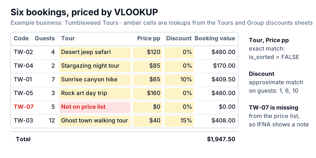
Five bookings price correctly, from $170.00 for two guests on the stargazing tour to $480.00 for four on the jeep safari. The sunrise hike for seven comes to 7 × $65 × 0.90 = $409.50, and the ghost town tour for twelve to 12 × $40 × 0.85 = $408.00.
Booking B-1045 shows #N/A. Its code, TW-07, is a tour that was never added to the price list. Wrap the lookups in IFNA so the sheet says what's wrong and totals still work:
=IFNA(VLOOKUP(C2, Tours!$A$2:$E$7, 2, FALSE), "Not on price list")=IFNA(VLOOKUP(C2, Tours!$A$2:$E$7, 4, FALSE), 0)
The month's total is $1,947.50 for the five priced bookings, and the sixth stands out for someone to fix. IFNA is better than IFERROR here because it only hides "not found". A broken formula still shows its error.
One formula for the whole column with ARRAYFORMULA
Copying a formula down works until someone adds a booking in row 8 and forgets to copy it again. Google Sheets has a cleaner option: put one formula at the top and let it fill the column.
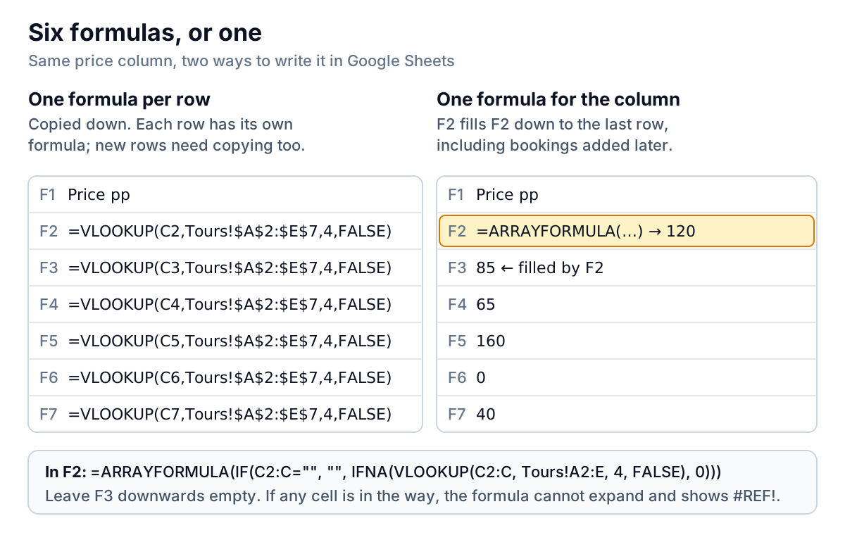
=ARRAYFORMULA(IF(C2:C="", "", IFNA(VLOOKUP(C2:C, Tours!A2:E, 4, FALSE), 0)))Reading it from the inside out:
VLOOKUP(C2:C, …)takes the whole tour code column as its search key, so it looks up every booking at once.Tours!A2:Ehas no end row. In Google Sheets an open-ended range runs to the bottom of the sheet, so new tours are included without editing the formula. You don't need dollar signs because the formula is never copied.IF(C2:C="", "", …)leaves rows without a booking blank instead of filling them with zeros.- ARRAYFORMULA lets functions that normally take one value work on a whole range and spill the results down. Pressing Ctrl+Shift+Enter while you edit a formula adds
ARRAYFORMULA(for you.
Two rules keep it working. Delete the old copied-down formulas first, because a full column needs empty cells below the formula: if anything is in the way, the formula can't expand and shows #REF!.
The practice workbook keeps one formula per row in the Solution tab so that it also works in Excel, which has no ARRAYFORMULA. Paste the version above into F2 once you've opened it in Sheets.
Looking up from another tab or another file
From another tab in the same spreadsheet, put the tab name and an exclamation mark in front of the range, as above. Google's guide to referencing other sheets says to add single quotes when the name contains spaces or other non-alphanumeric symbols: 'Group discounts'!A2:B4. Our VLOOKUP from another sheet guide covers what breaks these references in both Excel and Sheets.
From a different spreadsheet file, a plain reference doesn't work; Google says you must use IMPORTRANGE. Tumbleweed keeps its price list in its own file so that prices are changed in one place, and every bookings file reads from it:
=VLOOKUP(C2, IMPORTRANGE("https://docs.google.com/spreadsheets/d/…", "Tours!A2:E"), 4, FALSE)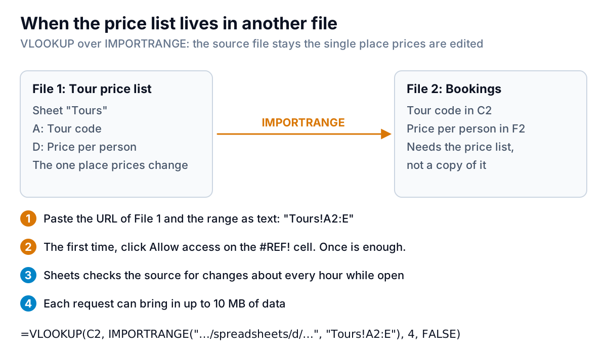
What Google's IMPORTRANGE help page says you should know:
- The URL and the range both go in quotation marks (or in cells you refer to). The sheet name in the range is optional and defaults to the first sheet, but name it anyway so adding a tab can't change what you import.
- The first time you connect two files, you're asked to allow access. After that, any editor of the bookings file can use IMPORTRANGE to pull from any part of the price list file, so think about who can edit the destination before you connect a file with sensitive data.
- Imports are capped at 10 MB of received data per request, and the function checks for updates every hour while the file is open. A price changed in the source may take a while to show.
- Chains of files that import from each other can cause long delays between updates.
If you have hundreds of rows each running their own IMPORTRANGE, a simpler setup is one IMPORTRANGE on a hidden tab (in A1: =IMPORTRANGE("…", "Tours!A1:E")) and ordinary VLOOKUPs pointing at that tab. Each lookup then reads a local range, and there's one connection to manage.
Lookups VLOOKUP can't do, and what to use in Sheets
Looking to the left. If a guide has the tour name and needs the code, which sits to its left on the Tours tab, build the range in the order you need with an array: =VLOOKUP("Rock art day trip", {Tours!B2:B7, Tours!A2:A7}, 2, FALSE) returns TW-05. Google's array help page explains the braces: commas put ranges side by side. In locales that use a comma as the decimal separator, you use a backslash instead.
XLOOKUP. Google Sheets has XLOOKUP, which searches any column and returns any other, exact match by default: =XLOOKUP(C2, Tours!A2:A7, Tours!D2:D7, "Not on price list"). Its fourth argument replaces IFNA. If the file will only ever be used in Sheets, it's the better choice for new formulas. See our XLOOKUP in Google Sheets guide.
Several conditions, or every match. VLOOKUP returns the first row for one key. To match on tour and date, or to list every booking for one tour, see VLOOKUP with multiple criteria; in Sheets, FILTER returns all matching rows.
Named ranges. Data > Named ranges lets you call Tours!A2:E7 something like tour_prices, as described in Google's named ranges guide. =VLOOKUP(C2, tour_prices, 4, FALSE) is easier to read and check.
Errors in Google Sheets and how to fix them
Most VLOOKUP Google Sheets errors fall into five patterns:
| You see | Likely cause in Sheets | Fix |
|---|---|---|
#N/A | The key isn't in the first column, or it's a number on one side and text on the other (common after a CSV import), or has a trailing space | Check the code exists; clean the column with TRIM; convert with VALUE or TO_TEXT so both sides match |
| A wrong value, no error | is_sorted left out, so Sheets used approximate match | Add FALSE |
#REF! | Index larger than the number of columns in the range; an ARRAYFORMULA blocked by data below it; IMPORTRANGE not yet allowed | Recount the columns; clear the cells below; click Allow access |
#VALUE! | Index is not a number, or less than 1 | Use a whole number of 1 or more |
#NAME? | Text typed into the formula without quotes | Write "TW-02", not TW-02 |
The VLOOKUP not working guide goes through each cause with examples, including invisible characters, and the full VLOOKUP guide covers column numbers and approximate match in more depth.
Once bookings are priced, the next step is usually a summary: revenue by tour, guests by week, which tours fill and which don't, the same questions a sales report answers. You can build that yourself with a Google Sheets dashboard. Or connect the sheet to Parity, which reads Google Sheets directly and builds a dashboard with headline numbers and trends, charts and a table of what needs attention, checking every number against queries on the full data first. You refine it by chat and share a read-only link with a business partner.
Connect the Google Sheet you already keep, and get revenue by tour and the bookings that need attention on one page. Build a report from your data free
Whichever you choose, the VLOOKUP Google Sheets habits that matter most are short: keep the price list in one place, keep FALSE at the end of every lookup on codes, and let IFNA tell you which bookings need a second look.