If VLOOKUP returns #N/A for a value you can see in the list, the two values aren't really identical: most often one is a number stored as text, or one has a hidden space, and =VLOOKUP(VALUE(TRIM(A2)), Items!$A$2:$E$14, 4, FALSE) fixes both. If it returns a number that's wrong, check the end of the formula first: without FALSE, VLOOKUP uses approximate match and returns a neighbouring row without any error.
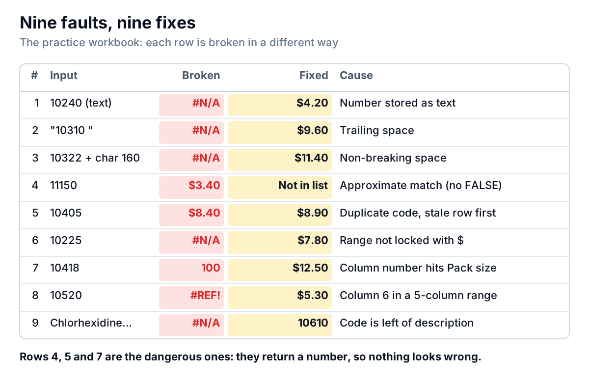
Those two cover most cases of VLOOKUP not working. The rest of this guide is a diagnosis table for every other cause, worked through on one example business: Osprey Vet Supply, a fictional distributor of veterinary consumables, looking up unit costs for a reorder. Download the practice workbook (.xlsx). Its Practice sheet has nine VLOOKUPs, each broken in a different way, with a blank column for your fix; the Solution sheet has the fixes, the causes and a quick check for each row.
The one-minute check before anything else
Pick a lookup that fails, find the row in the source list that you're sure it should match, and type a comparison in any empty cell. For Osprey, the item code is in C2 of the reorder sheet and the matching item sits in A4 of the Items sheet:
=C2=Items!A4If that says FALSE, VLOOKUP is right and your data is wrong: the two cells differ in a way you can't see. Two more formulas tell you how:
=ISTEXT(C2)and=ISTEXT(Items!A4). If one says TRUE and the other FALSE, one is text and one is a number.=LEN(C2). If an item code of five digits has a length of 6, there's a hidden character.
If the comparison says TRUE and VLOOKUP still fails, the problem is in the formula: the range, the column number or the last argument. Microsoft's Evaluate Formula tool (Formulas tab, Formula Auditing group) steps through it one part at a time so you can see which piece goes wrong.
VLOOKUP not working: the diagnosis table
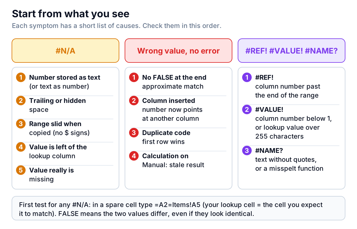
Most causes below can be reproduced in the practice workbook; the numbers in brackets in the Fix column are the matching fault numbers on its Practice sheet.
| Symptom | Cause | How to confirm | Fix |
|---|---|---|---|
#N/A | Lookup value is text, list holds numbers (or the reverse) | ISTEXT differs; text sits at the left of the cell | VALUE(C2) in the formula, or convert the column (row 1) |
#N/A | Trailing or leading space | LEN is one too long | TRIM(C3), plus VALUE if codes are numbers (row 2) |
#N/A, TRIM doesn't help | Non-breaking space (character 160) | =UNICODE(RIGHT(C4,1)) returns 160 | SUBSTITUTE(C4, UNICHAR(160), "") (row 3) |
#N/A lower down only | Range not locked; it slid when copied | Click the cell: the range starts below the item you want | Add dollar signs: Items!$A$2:$E$14 (row 6) |
#N/A | The value you have is to the right of the one you want | Your lookup column isn't the first column of the range | INDEX and MATCH, or XLOOKUP (row 9) |
#N/A | The value really isn't in the list | COUNTIF on the list returns 0 | Add it, or show a message with IFNA |
| Wrong value, no error | Last argument missing or TRUE, so approximate match | Formula ends with 4) or TRUE) | End with FALSE) (row 4) |
| Wrong value, no error | Duplicate key; first row wins | COUNTIF returns 2 or more | Remove the stale row (row 5) |
| Wrong value, no error | A column was inserted or deleted | Result belongs to the column next door | Use MATCH on the header for the column number (row 7) |
| Old value that won't update | Calculation set to Manual | Changing the source doesn't change the result | Set calculation to Automatic, or press F9 |
#REF! | Column number bigger than the range is wide | Count the columns in the range | Correct the number (row 8) |
#VALUE! | Column number below 1, or lookup value over 255 characters | Check the third argument; check LEN | Fix the number; use INDEX/MATCH for long text |
#NAME? | Text in the formula without quotes, or a misspelt name | Look for bare words in the formula | "10240" in quotes, or retype the name |
| Formula shows as text | The cell was formatted as Text before you typed | The cell shows =VLOOKUP(… instead of a result | Format as General, click in the cell, press Enter |
Microsoft's own troubleshooting pages for the #N/A error and the #VALUE! error cover the same ground; the VLOOKUP reference lists #REF!, #NAME? and #SPILL!.
#N/A when the value is right there
Numbers stored as text
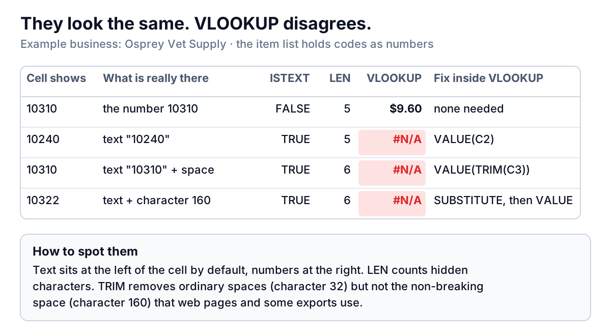
This is the classic. Osprey's item list holds codes as numbers. The reorder list came from a stock-count export, where the same codes arrived as text. 10240 and "10240" look identical, but VLOOKUP treats them as different values, so it returns #N/A.
Fix it inside the formula with =VLOOKUP(VALUE(C2), Items!$A$2:$E$14, 4, FALSE), which returns $4.20. If the text is in the list rather than the lookup cell, go the other way and turn the number into text: C2&"". Better still, fix the column once. Microsoft's guide to converting numbers stored as text gives three ways: the error indicator's Convert to Number option, the VALUE function in a helper column, or Paste Special with Multiply by 1.
Spaces you can't see
Exports from tills, accounting tools and web pages often add a space after a code or a name. "10310 " has a length of 6 and doesn't match 10310. TRIM removes leading and trailing spaces; wrap it in VALUE when the list holds numbers: =VLOOKUP(VALUE(TRIM(C3)), Items!$A$2:$E$14, 4, FALSE) returns $9.60.
When TRIM doesn't help, the space is probably a non-breaking one. Microsoft's TRIM reference says it was designed to trim the ordinary space (character 32) and that the non-breaking space, character 160, is a different character that web pages use. Remove it by name: =VLOOKUP(VALUE(SUBSTITUTE(C4, UNICHAR(160), "")), Items!$A$2:$E$14, 4, FALSE) returns $11.40. UNICHAR works in Excel 2016 and later on Windows and Mac. If a whole export is full of these, clean the column once rather than patching every formula; our guide to cleaning data in Excel shows how.
The range slid down
The formula in row 2 worked, so it was copied down. Without dollar signs, Items!A2:E14 became Items!A7:E19 by row 7, and item 10225, which sits in row 3 of the item list, is no longer inside the range. Lock it with dollar signs (press F4 while the cursor is on the range) and copy it down again.
The value you want is to the left
VLOOKUP only searches the first column of the range and only returns columns to its right. Osprey's buyer has a description, "Chlorhexidine scrub 4% 500 ml", and wants the item code from column A. No column number fixes that. Use =INDEX(Items!$A$2:$A$14, MATCH(C10, Items!$B$2:$B$14, 0)), which returns 10610, or XLOOKUP if you have it (Microsoft 365 and Excel 2021 or later).
A number comes back, and it's wrong
These are the dangerous ones, because nothing on the sheet looks broken.
Approximate match. The fourth argument is optional, and when it's missing, Excel uses approximate match. On a sorted list, a code that isn't there returns the row with the next smaller code. Osprey's buyer typed 11150 for an Elizabethan collar; there's no such code, so =VLOOKUP(C5, Items!$A$2:$E$14, 4) returned $3.40, the cost of item 11140. With FALSE it shows #N/A, and with IFNA(…, "Not in item list") it says so in words. Our VLOOKUP guide explains when approximate match is the right choice.
Duplicate keys. Item 10405, 3 ml syringes, appears twice in the list: last year's row at $8.40 above this year's at $8.90. VLOOKUP returns the first, so every reorder line is costed at the old price. Find duplicates with =COUNTIF(Items!$A$2:$A$14, C6) (anything above 1) and delete the stale row. If you can't change the list and you have Microsoft 365 or Excel 2021 or later, =XLOOKUP(C6, Items!$A$2:$A$14, Items!$D$2:$D$14, "Not found", 0, -1) searches from the bottom up and returns $8.90.
The column moved. Someone inserted a Pack size column in the item list. The formula still says column 3, so it now returns 100 (a box of 100) instead of a cost of $12.50. Find the column by its header instead: MATCH("Unit cost", Items!$A$1:$E$1, 0) in place of the 3.
Calculation is set to Manual. A workbook set to manual calculation doesn't update formulas when data changes, and the setting can arrive with a file someone else saved. Microsoft's guide to recalculation options shows where to switch it back to Automatic (File > Options > Formulas); F9 recalculates in the meantime.
Errors that point at the formula itself
#REF!: the column number is larger than the number of columns in the range. Osprey's range is five columns wide, so column 6 can't exist. It also appears when a sheet or file the formula refers to has been deleted; see VLOOKUP from another sheet for links that break.#VALUE!: the column number is less than 1, or the lookup value is more than 255 characters. For long text, Microsoft suggests INDEX and MATCH.#NAME?: usually text typed into the formula without quotation marks, such as=VLOOKUP(Gauze, …). It also appears when someone opens a file containing XLOOKUP in Excel 2019 or earlier.#SPILL!: in Microsoft 365, using a whole column such asA:Aas the lookup value tries to return a result for every row. Use a single cell, or put@in front of the column, as the VLOOKUP reference describes.
Two odd ones. If your lookup value contains an asterisk or question mark, VLOOKUP treats them as wildcards with exact match, so "Bandage 10cm*" matches anything starting with "Bandage 10cm". Put a tilde in front (~*) to search for the character itself. And if the formula cell shows the formula as text instead of a result, the cell was formatted as Text when you typed it.
Stop it happening next month
Six habits prevent nearly every case of VLOOKUP not working that this guide covers:
- End every lookup on codes or names with
FALSE. - Lock ranges with dollar signs, or point at a table that grows.
- Use MATCH on the header instead of a typed column number.
- Clean imported columns once (TRIM, convert to numbers) before you look anything up.
- Wrap with IFNA rather than IFERROR, so only "not found" is hidden, then count how many:
=COUNTIF(E2:E50, "Not in item list"). - Check the key column for duplicates with COUNTIF whenever the list is replaced.
Most broken VLOOKUPs in a small business trace back to the same job: matching an export from one system to a list from another every month, such as stock counts against an item master, or an invoice list exported from one of the QuickBooks reports against a customer list. If that's the work, Parity can build the report from the exports directly. Upload the files as CSV or Excel and it builds a dashboard with headline numbers, charts and a table of what needs attention, and every number is checked against queries on the full dataset before you see it. For stock in particular, our inventory dashboard guide shows what's worth tracking once the lookups work.
Upload your stock count and item list, and get a checked dashboard of stock and reorder costs. Build a report from your data free
And the next time you find VLOOKUP not working, go back to the one-minute check: compare the two cells directly, and let ISTEXT and LEN tell you which kind of different they are.