Here's how to clean data in Excel. Work through it in a fixed order: delete rows that aren't records, strip spaces with TRIM, turn text into numbers with VALUE or NUMBERVALUE, turn text into dates with DATE, split combined columns, make labels consistent, then check your total against the source. Do each fix in a new column beside the raw data, not on top of it, so you can see what changed and undo any of it.
The order matters because each step depends on the one before. You can't convert "$1,240.00 " to a number while it still has a trailing space, and you can't trust a total until the Total row from the export is gone. This guide walks through how to clean data in Excel using one real-looking export from Anchor Point Marine, an example marine parts shop, with every formula you need and a check after each step.
Download the practice workbook (.xlsx). It has the raw export, a Practice sheet with the clean columns left empty, and a Solution sheet with every formula and before-and-after checks.
What a messy export does to your numbers
Anchor Point Marine exported its online orders for 1 to 6 September: eight orders, six columns (Order, Created at, Customer, Item, Amount, Status), with every column stored as text. The export ends with a blank row and a Total row showing $2,998.75. It looks fine on screen. Then the owner tries to use it.
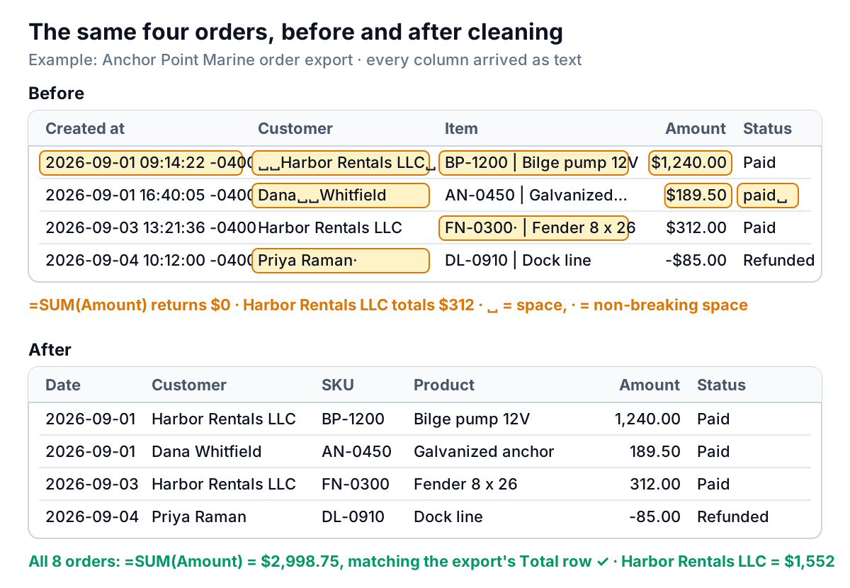
=SUM(E2:E9)returns 0, because "$1,240.00" stored as text isn't a number.=SUMIFS(M2:M9,C2:C9,"Harbor Rentals LLC")returns $312, not $1,552, because one of Harbor Rentals' two orders has the name typed as " Harbor Rentals LLC " with spaces around it.- Paid orders come to $2,610, not $2,799.50, because one status is "paid " with a trailing space.
- A lookup on SKU FN-0300 fails, because there's an invisible non-breaking space after it.
- Sorting by date sorts text, not dates.
None of this shows as an error. Every formula returns a believable number. That's why cleaning comes before any pivot table, chart or report.
How to clean data in Excel, step by step
Microsoft's own checklist, Top ten ways to clean your data, starts with two habits worth copying: keep a backup copy of the original in a separate workbook, and make sure the data is in a table layout, with similar data in each column and no blank rows. Then work in this order:
1. Remove rows that aren't records
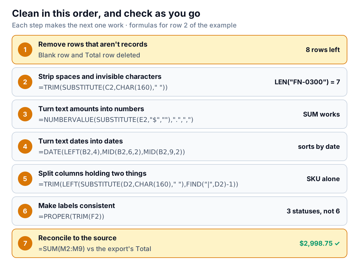
Exports often add blank rows, repeated headers, subtotals or a grand total. Leave the Total row in and, once the amounts are numbers, every sum counts it: Anchor Point's six days would show $5,997.50, twice the real figure. Filter each column for blanks and for words like "Total", and delete those rows. Anchor Point is left with 8 rows. Note the export's Total ($2,998.75) somewhere first; you'll need it in step 7.
2. Strip spaces and invisible characters
TRIM removes all spaces except single spaces between words, so " Harbor Rentals LLC " becomes "Harbor Rentals LLC" and "Dana Whitfield" becomes "Dana Whitfield". But Microsoft's TRIM page is explicit that it only removes the ordinary space (character 32). The non-breaking space (character 160), common in data copied from web pages and some exports, survives. Replace it first:
=TRIM(SUBSTITUTE(C2,CHAR(160)," "))For line breaks and other non-printing characters, wrap it in CLEAN, which Microsoft's top-ten page says removes the first 32 non-printing characters in the 7-bit ASCII code. The check is LEN: "FN-0300" should be 7 characters. Before cleaning, Anchor Point's comes out at 8.
3. Turn text amounts into numbers
Spot text numbers with a count: =COUNT(E2:E9) counts numbers and returns 0, while =COUNTA(E2:E9) counts anything and returns 8. Text numbers also tend to sit left-aligned, and Excel may mark plain ones with a green triangle. Microsoft's guide to converting numbers stored as text covers that error indicator (select the cells, click it, choose Convert to Number) and the VALUE function.
For amounts with currency symbols and thousands separators, NUMBERVALUE is safer, because you tell it which character is the decimal point and which groups thousands instead of relying on your computer's regional settings. Microsoft's NUMBERVALUE page gives the syntax as NUMBERVALUE(Text, [Decimal_separator], [Group_separator]):
=NUMBERVALUE(SUBSTITUTE(E2,"$",""),".",",")"$1,240.00" becomes 1240 and "-$85.00" becomes -85. For a European-style export ("2.500,27"), swap the separators: =NUMBERVALUE(E2,",","."). If you see #VALUE!, there's a character left that isn't a digit, separator or sign; check for a currency code like "USD" and remove it with another SUBSTITUTE.
4. Turn text dates into dates
The export's "2026-09-01 09:14:22 -0400" is text. Microsoft's DATEVALUE function converts text in a date format Excel recognises, and ignores any time in it. When an export uses a fixed layout, building the date from its parts is more dependable, because it doesn't depend on how your copy of Excel reads dates:
=DATE(LEFT(B2,4),MID(B2,6,2),MID(B2,9,2))Year from characters 1–4, month from 6–7, day from 9–10. Format the column as a date. The check: =COUNTIFS(I2:I9,">="&DATE(2026,9,1),I2:I9,"<"&DATE(2026,10,1)) should return 8, every order in September. If your export uses day/month/year text such as "03/09/2026", the same idea works with the positions changed; the danger is converting it with a method that guesses, and getting 9 March.
5. Split columns that hold two things
"BP-1200 | Bilge pump 12V" is a SKU and a product name in one cell. Microsoft's Convert Text to Columns Wizard does it with clicks: select the column, Data > Text to Columns, choose Delimited, enter | under Other, choose a destination, and Finish. Pick an empty destination, or it can write over the columns to the right. Then trim the results.
Formulas keep it live:
=TRIM(LEFT(SUBSTITUTE(D2,CHAR(160)," "),FIND("|",D2)-1))— the SKU
=TRIM(MID(D2,FIND("|",D2)+1,100))— the product name
In Microsoft 365 and Excel 2024, TEXTSPLIT does it in one formula, =TEXTSPLIT(D2," | "), spilling the two parts into neighbouring cells. Microsoft describes it as the Text to Columns wizard in formula form. If a row has no "|", FIND returns #VALUE!; wrap the formula in IFERROR(…,D2) or fix the row.
One warning: keep codes as text. If your SKUs or ZIP codes have leading zeros ("00450"), converting them to numbers drops the zeros, and lookups against your product list stop matching.
6. Make labels consistent
The Status column has "Paid", "paid " and "PAID" for the same thing, plus "Pending" and "pending". =PROPER(TRIM(F2)) turns six spellings into three statuses: Paid, Pending and Refunded. UPPER and LOWER are the alternatives. Don't run PROPER on customer names, though: it turns "Harbor Rentals LLC" into "Harbor Rentals Llc".
Does case matter? For SUMIFS and COUNTIF, no: Microsoft's COUNTIF guide says criteria aren't case-sensitive, so "PAID" already matched "Paid". The trailing space in "paid " is what broke it. For Power Query, yes: Microsoft warns that it's case-sensitive.
7. Reconcile to the source
This is the step people skip. Sum the cleaned amounts and compare with the export's own Total: =SUM(M2:M9) returns $2,998.75, which matches. Check the row count (8) and one or two numbers you know, such as Harbor Rentals at $1,552. If the total is off, filter the cleaned amount column for errors or blanks; one row that didn't convert is the usual cause.
Once everything checks out, copy the clean columns, paste them back with Paste Special > Values, and delete the raw columns. Microsoft's top-ten page recommends the same pattern: a new column with the formula, converted to values, with the original removed.
Power Query: clean once, refresh every month
If the same export arrives every month, record the steps instead of repeating them. Power Query is built into current Excel. Load the data with Data > From Table/Range, or Data > Get Data for a file; Microsoft's guide to creating a query covers both. Each change you make is saved as an applied step.
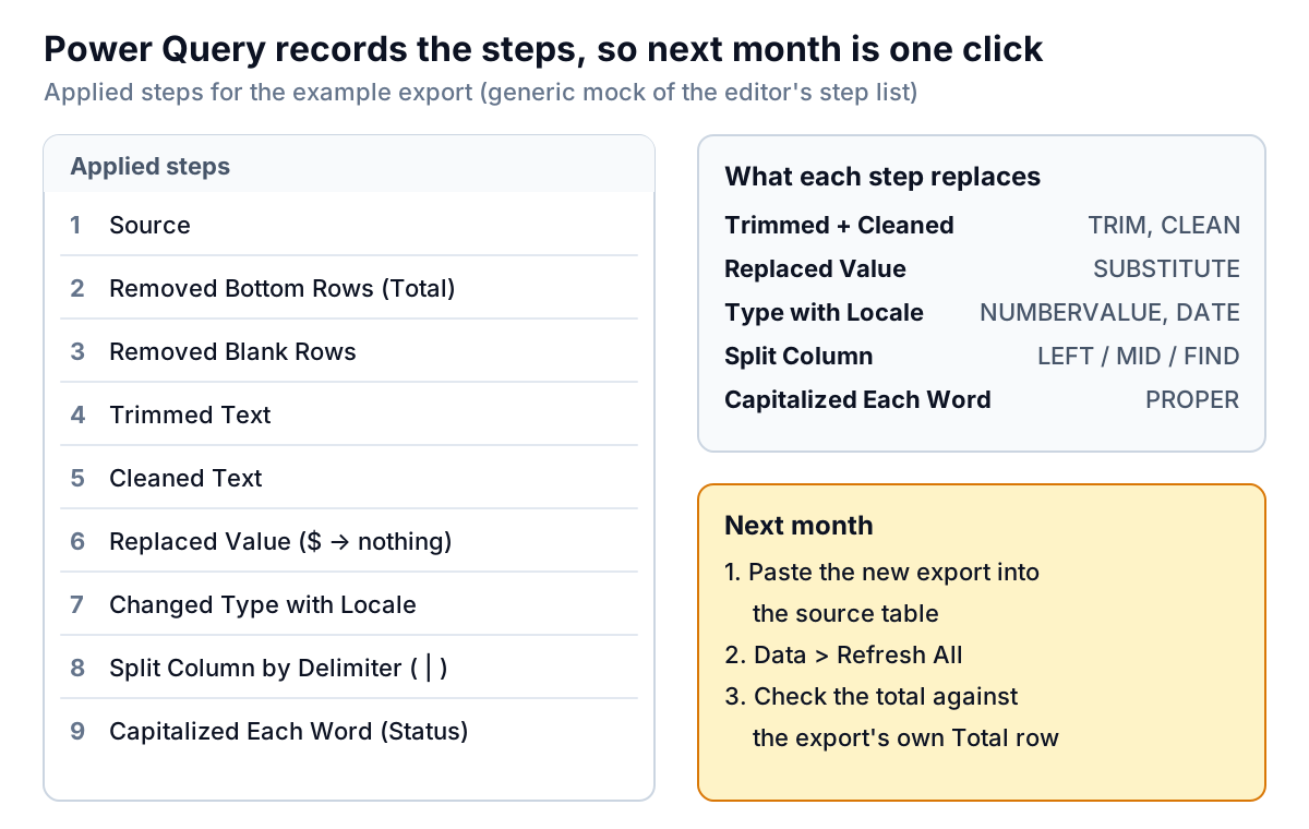
- Remove the Total and blank rows: Home > Remove Rows has Remove Bottom Rows and Remove Blank Rows (see Microsoft's article on filtering by row position).
- Trim and clean: select the text columns, then Transform > Format > Trim, and Format > Clean.
- Remove the $ sign: Replace Values, with "$" replaced by nothing. Microsoft's Replace values article notes that text columns get advanced options, including special characters.
- Split Item: Split Column > By Delimiter, using " | " (Microsoft's guide to splitting columns by delimiter shows where it lives on the Home and Transform tabs).
- Set types: click the type icon in each column header, or Home > Data Type. For amounts or dates written in another region's style, choose Using locale at the bottom of the list, as Microsoft's page on adding or changing data types describes.
- Close & Load, then check the total against the export, as in step 7.
Next month, paste the new rows into the source table, or replace the file, and choose Data > Refresh All. One caution from that same Microsoft page: Power Query automatically adds a "Changed Type" step when it loads data, and that guess can cause refresh errors later, for example when a column that was all numbers gets a text value. If a refresh fails, look at that step first.
Mistakes that undo your cleaning
Most of what goes wrong when people learn how to clean data in Excel comes from a few habits:
| Mistake | What happens | Do this instead |
|---|---|---|
| Cleaning on top of the raw data | No way to check or undo after saving | Clean in new columns; keep the original export untouched |
| Find and Replace across the whole sheet | Replacing "-" to fix dates also wrecks SKUs like "BP-1200" | Select one column first |
| Using TRIM alone on web or exported text | Non-breaking spaces survive; lookups still fail | TRIM(SUBSTITUTE(x,CHAR(160)," ")) |
| Text to Columns into occupied cells | Overwrites the next columns | Insert empty columns or set a destination |
| Converting codes to numbers | "00450" becomes 450 | Keep SKUs, ZIP codes and phone numbers as text |
| Leaving the Total row in | Every total doubles | Remove it first, then reconcile to it |
| Removing duplicates before cleaning | "Harbor Rentals LLC" and " Harbor Rentals LLC " count as two | Clean, then dedupe (see how to remove duplicates in Excel) |
If you clean the same exports every month
Most small businesses clean the same two or three files every month: an online store export, a payments report, an accounting export. Our guides to Shopify reports and QuickBooks reports show which reports are worth exporting in the first place. If the cleaning is just a step on the way to a monthly summary, Parity can take that step off your list. Upload the CSV or Excel export, or connect Shopify, QuickBooks Online, Stripe, Square, HubSpot or Google Sheets directly, and it builds a dashboard: headline numbers with trends, charts, what explains them, and a table of what needs attention. Every number is checked against queries on the full dataset before you see it. If something looks off, ask it in plain words ("treat 'paid ' and 'PAID' as Paid") and refine with versions and undo. Next month, update it with the new file. Parity doesn't read PDFs, so start from the CSV or Excel export.
Upload last month's export and see the dashboard Parity builds from it. Build a report from your data free
If you stay in Excel, keep the order: rows, spaces, numbers, dates, splits, labels, then reconcile. Anchor Point's file went from a $0 total to $2,998.75 that matches the source, and the last step is the one that proves it.