To remove duplicates in Excel, select any cell in your list, go to Data > Data Tools > Remove Duplicates, tick only the columns that define a repeat, and click OK. Excel keeps the first row of each set, deletes the rest, and tells you how many it removed and how many unique values remain.
That's the whole button. Knowing how to remove duplicates in Excel correctly comes down to which columns you tick and which row comes first, and that's what most guides skip. Silverline Events, an example event-planning business we'll use throughout, merged two lists of enquiries and got 14 rows worth $103,600 in quotes. Only 8 were real enquiries, worth $58,350. Depending on how you remove duplicates in Excel, you can end up with 13, 9 or 8 rows from that same list. Only one of those is right.
Download the practice workbook (.xlsx). It has Silverline's 14 rows, a Practice sheet with empty helper columns, and a Solution sheet with every formula below filled in and checked.
Decide what a duplicate is before you click anything
Silverline's list came from two places: the enquiry form on its website and a spreadsheet the coordinator kept from phone calls and emails. It has six columns: Received, Client, Email, Event date, Guests and Quote. Some repeats are obvious. Others aren't repeats at all.
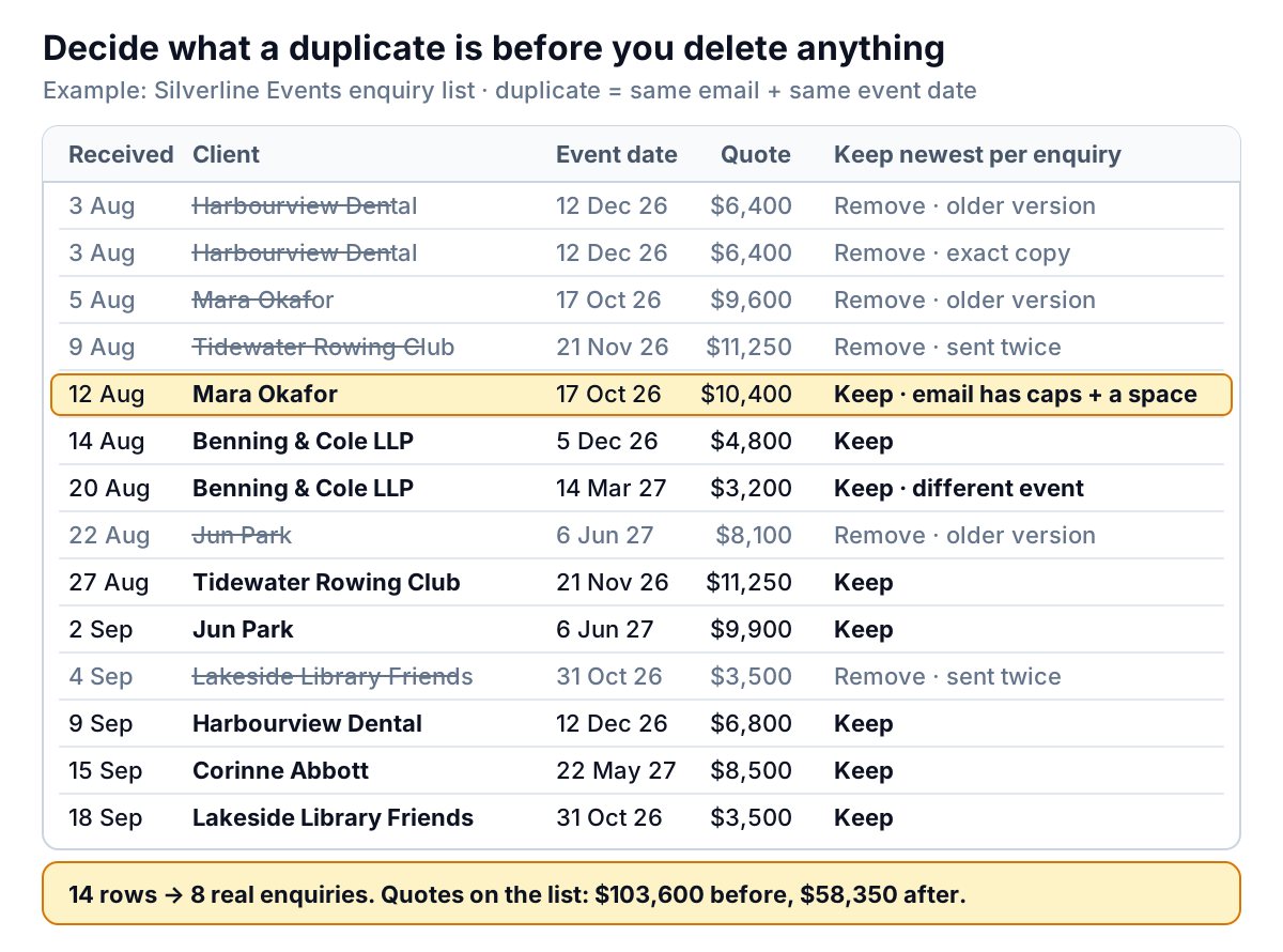
Look at the kinds of repeat in that list:
- Exact copies. Harbourview Dental's form was submitted twice on 3 August. Every cell matches.
- The same enquiry sent twice. Tidewater Rowing Club appears on 9 August and again on 27 August with the same details. Only the Received date differs.
- Updated versions. Jun Park first asked about 90 guests ($8,100), then came back with 110 ($9,900). The newer row is the one you want.
- Repeats hiding behind formatting. Mara Okafor's second email is typed
Mara.Okafor@mail.example, with capitals and a trailing space. - Not a duplicate. Benning & Cole LLP enquired about a December party and a March event. Same client, two jobs.
So Silverline's rule is: one enquiry is one email address plus one event date, and if it appears more than once, keep the most recently received row. Write your own rule down in one sentence before you start. It tells you which columns to tick, whether you need to clean anything first, and which row should survive.
How to remove duplicates in Excel with the Remove Duplicates button
Microsoft's guide to filtering for unique values or removing duplicate values gives the steps:
- Copy the sheet first. Microsoft recommends copying the original range to another sheet or workbook, because removing duplicates permanently deletes rows. Ctrl+Z works straight away, but not after you've saved and closed.
- Click any cell in the list (or select the range) and choose Data > Data Tools > Remove Duplicates.
- Leave My data has headers ticked if row 1 holds column names.
- Under Columns, click Unselect All, then tick only the columns in your rule.
- Click OK. Excel shows how many duplicate values were removed and how many unique values remain.
Two details from Microsoft's page matter. First, the columns you tick only decide what's compared: whole rows are still deleted, including the columns you didn't tick. Second, Excel keeps the first occurrence and deletes the later ones. Whatever is on top wins.
Here's what Silverline's list gives you with three different choices:
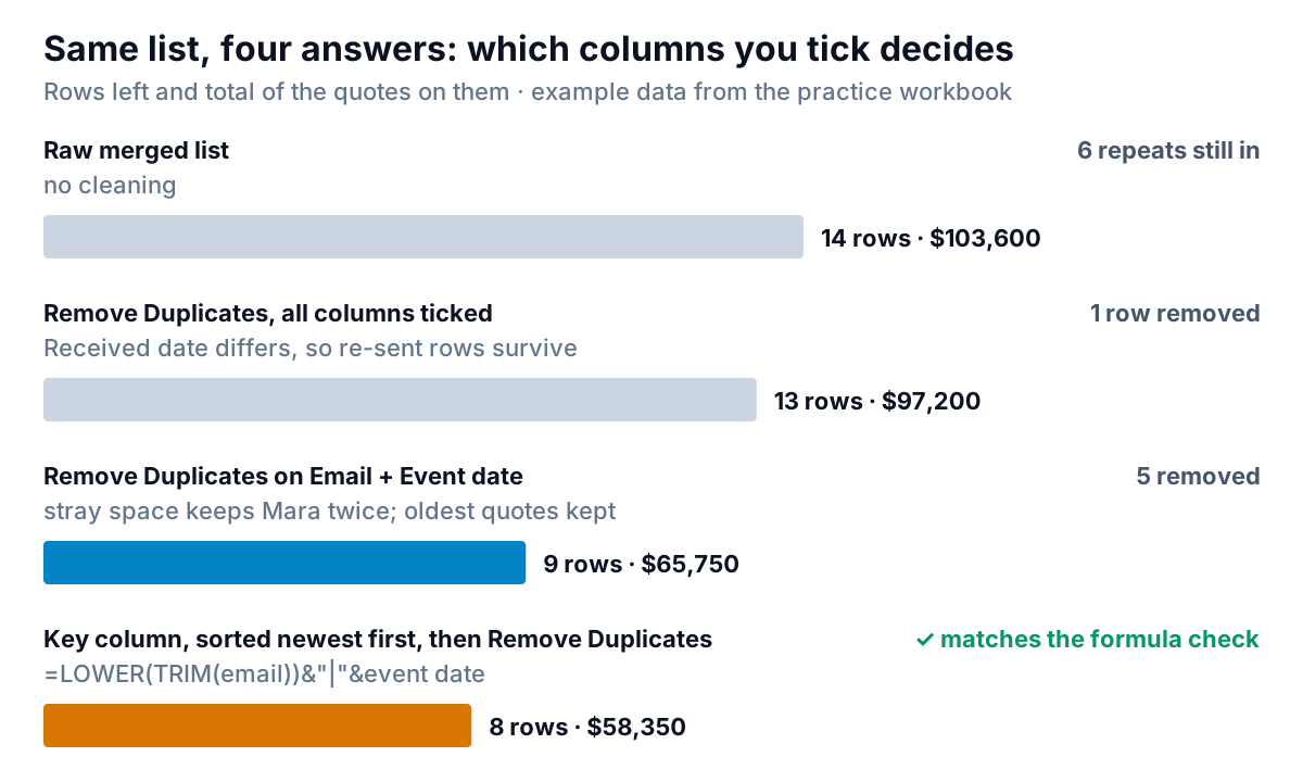
- All columns ticked removes one row: Harbourview's double submission. The other repeats survive because their Received dates differ.
- Email and Event date ticked removes five rows, but keeps Mara twice (the trailing space makes her two emails look different) and keeps the oldest quote for Harbourview ($6,400 instead of $6,800) and Jun Park ($8,100 instead of $9,900).
- A cleaned key, sorted newest first removes six rows and leaves exactly the 8 enquiries. The next two sections show how.
Highlight duplicates first, then delete
On a list you care about, look before you delete. The quick way is conditional formatting: select a column, then Home > Conditional Formatting > Highlight Cells Rules > Duplicate Values, the path Microsoft's page gives. Every repeated value gets coloured, so you can scan them.
That rule works cell by cell, though. Highlight the Email column on Silverline's list and Benning & Cole lights up, even though its two rows are different events. When your rule involves more than one column, build a helper column instead. In the practice workbook, column G joins the cleaned email and the event date into one key:
=LOWER(TRIM(C2))&"|"&D2TRIM strips the stray spaces, LOWER makes capitals irrelevant, and the | keeps the two parts apart so different combinations can't run together into the same text. The date joins as its serial number (46312 for 17 October 2026), which is fine for matching. Then count each key:
=COUNTIF($G$2:$G$15,G2)— how many times this key appears (Harbourview: 3)
=COUNTIF($G$2:G2,G2)— which occurrence this row is (1 for the first, 2 for the second…)
The second formula uses a range that grows as you fill it down: $G$2 is locked, G2 isn't. Filter the count column for anything above 1 and you see every repeat, with its partners, before anything is deleted. Microsoft's COUNTIF guide also warns that it returns wrong results for strings longer than 255 characters, and that leading or trailing spaces and non-printing characters cause unexpected results. Both are reasons to clean the key with TRIM.
Keep the latest row, not the first
Because Remove Duplicates keeps the first occurrence, you control which row survives by controlling the order.
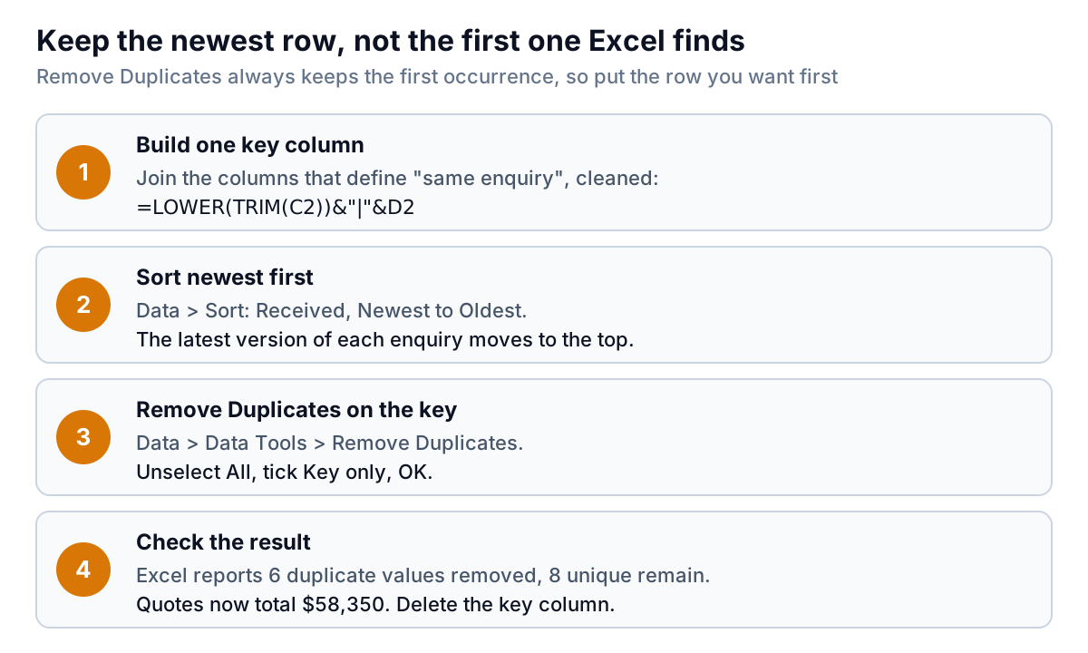
- Add the key column above.
- Sort by Received, newest to oldest (Data > Sort).
- Run Remove Duplicates with only the key column ticked.
- Check the count: Silverline should see 6 removed and 8 remaining, with quotes totalling $58,350.
If you'd rather mark rows than delete them, a formula can find the newest row for each key. MAXIFS returns the latest Received date per key, and Microsoft's MAXIFS page lists it for Excel 2019 and later and Microsoft 365:
=MAXIFS($A$2:$A$15,$G$2:$G$15,G2)
=IF(AND(A2=J2,COUNTIFS($G$2:G2,G2,$A$2:A2,A2)=1),"Keep","Remove")
The second formula says Keep when this row has the latest date for its key and is the first row with that key and date, which handles exact copies received on the same day. Filter for Remove and delete those rows, or leave them and filter them out. In the workbook, =SUMIFS(F2:F15,K2:K15,"Keep") returns $58,350, matching the Remove Duplicates result. On Excel 2016 or earlier, without MAXIFS, use the sort-newest-first method and keep rows where the occurrence number is 1.
UNIQUE: a duplicate-free list that updates itself
Not every answer to how to remove duplicates in Excel should delete anything. Remove Duplicates changes your data once. If you want a clean list next to the original that keeps up as rows are added, use the UNIQUE function. Microsoft lists it for Microsoft 365, Excel 2024, Excel 2021 and Excel on the web and mobile. Excel 2019 and earlier don't have it.
=UNIQUE(array, [by_col], [exactly_once])=UNIQUE(G2:G15)returns Silverline's 8 keys in one go. The results "spill" down into the cells below.=UNIQUE(B2:B15)lists each client once: 7 names, because Benning & Cole's two events share one name.=SORT(UNIQUE(B2:B15))gives the same list in A–Z order. SORT has the same version requirements.=UNIQUE(B2:B15,,TRUE)sets exactly_once, returning only clients that appear exactly once. Silverline gets one name, Corinne Abbott. That's useful for the opposite question: who enquired once and never came back?=ROWS(UNIQUE(G2:G15))counts distinct enquiries: 8.
Two errors come up. #SPILL! means something is in the way of the results; Microsoft's guide to fixing a #SPILL! error shows how to select the obstructing cells. #NAME? usually means the file has been opened in a version without UNIQUE. Microsoft also notes that dynamic arrays between workbooks have limited support: a UNIQUE formula pointing at another workbook returns #REF! when that workbook is closed. Point it at a table in the same file.
On older versions, Data > Sort & Filter > Advanced, with Copy to another location and Unique records only ticked, copies a duplicate-free list elsewhere without touching the original. It's a one-off copy, not a live formula.
Power Query, when the list arrives every month
If Silverline gets a fresh export every month, repeating these steps by hand gets old. Power Query records them once. Select the list, choose Data > From Table/Range (Microsoft's guide to creating a query explains the options), and then, in the Power Query Editor:
- Select the Email column and use Transform > Format > lowercase, then Format > Trim.
- Sort Received descending.
- Select Email and Event date, then Home > Remove Rows > Remove Duplicates, as described in Microsoft's article on working with duplicate values.
- Close & Load. Next month, paste the new rows into the source table and choose Data > Refresh All.
Two warnings from that same Microsoft page. Power Query is case-sensitive, so "Mara.Okafor" and "mara.okafor" are different unless you lowercase first, which is why step 1 comes before step 3. And Power Query doesn't guarantee it keeps the first instance in a set of duplicates, so sorting newest first isn't a reliable keep-latest method on its own. Microsoft's note on preserving sort covers the fix, which uses Table.Buffer on the sorted step. If that's more than you want to manage, use the MAXIFS Keep column in the sheet and filter on it in Power Query instead.
There's also Home > Keep Rows > Keep Duplicates, which does the reverse: it shows only the rows that repeat. It's a quick way to review them before you remove anything.
Why duplicates survive: the usual causes
If you removed duplicates and some are still there, it's almost always one of these:
| What you see | Cause | Fix |
|---|---|---|
| Two rows look identical but both stay | Trailing or double spaces, or a non-breaking space from a web export | Clean into a key with TRIM; for non-breaking spaces, TRIM(SUBSTITUTE(C2,CHAR(160)," ")) |
| Same date, both rows kept | Different date formats, or one date stored as text | Format the column one way; convert text dates first |
| Same order number, both kept | One is a number, the other is text that looks like a number | Convert the text numbers first (see our guide to cleaning data in Excel) |
| Re-sent enquiries survive | A timestamp or Received column was ticked | Tick only the columns in your rule |
| Wrong version kept | Excel keeps the first occurrence | Sort so the row you want is first |
| Real records deleted | Too few columns ticked (Client alone would merge Benning & Cole's two events) | Undo straight away, or go back to your copy |
| Remove Duplicates won't run | The data is outlined or has subtotals | Remove subtotals, then try again |
After any removal, check a total. Count the rows and sum the money column before and after, and make sure the difference is what you expected. Silverline's should drop by 6 rows and $45,250. A quick pivot table by client is another good check; if a name appears twice, something about it differs. Our sales report guide has more checks like these for the numbers that go to your accountant or partner.
When duplicates come from combining exports
Silverline's problem is typical: duplicates rarely start in one system. They appear when two exports are stacked together, such as an online store and a till, a CRM and a form tool, or two months of the same report that overlap by a few days. If you're doing this every month to build one view of sales or enquiries, Parity can take the CSV or Excel exports directly, or connect Shopify, Square, HubSpot, QuickBooks Online, Stripe or Google Sheets, and build a dashboard from them: headline numbers with trends, charts, what explains them, and a table of what needs attention. Every number is checked against queries on the full dataset before you see it, and you can ask it in plain words to count each order once. Update it with next month's file instead of redoing the steps, or see our Excel dashboard guide if you'd rather keep it in a workbook.
Upload your exports and get a checked dashboard built from them. Build a report from your data free
Whichever method you choose for how to remove duplicates in Excel, the rule comes first. Write down what makes two rows the same and which one should survive. The clicks are the easy part.