VLOOKUP: How to Use It, With Worked Examples and Fixes

To pull a price, name or cost from a list into another table, type =VLOOKUP(B2, Products!$A$2:$E$11, 4, FALSE): find the value in B2 in the first column of the price list, then return what sits in the 4th column of that row. Get the last argument right (FALSE for an exact match) and lock the range with dollar signs, and VLOOKUP will fill an order, an invoice list or a stock sheet in seconds.

This guide walks through VLOOKUP on one example business, Pinecrest Pet Supply, a fictional pet shop pricing a trade order from its product list. Every number in it can be reproduced in the workbook. Download the practice workbook (.xlsx): the Practice sheet has the formula cells blank, and the Solution sheet has them filled in.

What VLOOKUP does, one argument at a time

VLOOKUP looks down the first column of a table until it finds what you asked for, then reads across that row to the column you name. Microsoft's VLOOKUP reference gives the syntax as VLOOKUP(lookup_value, table_array, col_index_num, [range_lookup]). It works in every desktop version of Excel still in use, including Excel 2016, 2019, 2021, 2024 and Microsoft 365, and Google Sheets has the same function with slightly different argument names.

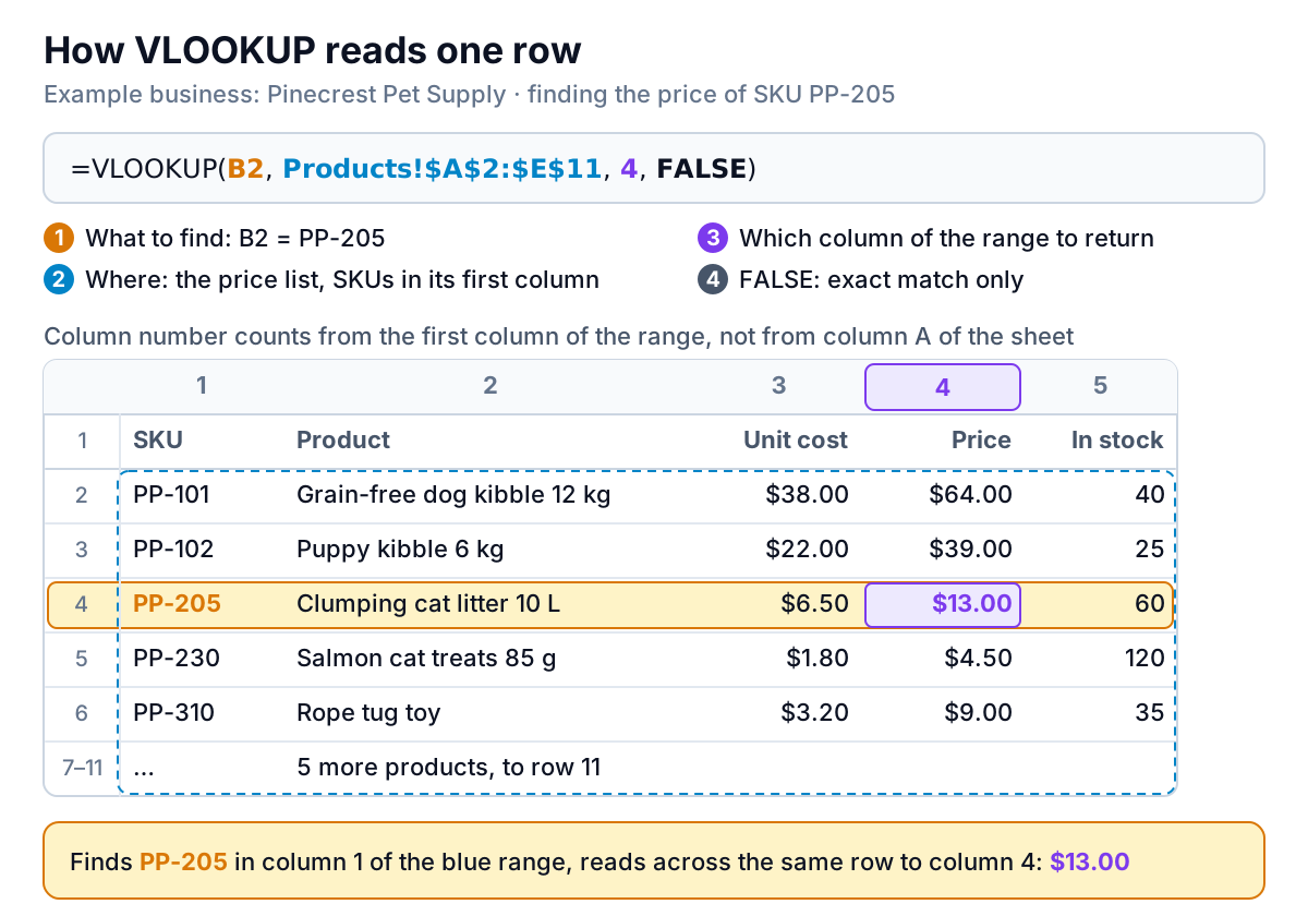
1. lookup_value: what you're looking for. Usually a cell on the same row, such as the SKU in B2. It must appear in the first column of the table.
2. table_array: the block of data to search, starting at the column that holds the lookup values and running at least as far right as the column you want back. Pinecrest's price list is Products!$A$2:$E$11: SKU, product, unit cost, price and stock for ten products.
3. col_index_num: which column of that block to return, counting the first column as 1. Price is the 4th column, so it's 4.
4. range_lookup: FALSE for an exact match, TRUE for an approximate one. It's optional, and if you leave it out Excel uses TRUE. That default causes more wrong answers than anything else in this guide, so the next sections cover it in detail.

Build your first VLOOKUP: prices into an order

Pinecrest's trade order sheet has five lines: a SKU in column B and a quantity in column C. The product name, price and line total are blank. Here's how to fill them, step by step.

1. Click the first empty price cell (E2) and type =VLOOKUP(.
2. Click the SKU cell B2, then type a comma.
3. Switch to the Products sheet and drag across the whole price list, A2 to E11. Press F4 once so the range becomes $A$2:$E$11. Microsoft's guide to relative, absolute and mixed references explains why: without the dollar signs, the range moves down one row every time you copy the formula down, and lines near the bottom of the order stop finding products near the top of the list.
4. Type the column number, 4, and a comma.
5. Type FALSE, close the bracket and press Enter. E2 shows $13.00, the price of PP-205 clumping cat litter.
6. Copy the formula down to E6. B2 changes to B3, B4 and so on because it has no dollar signs; the range stays put because it does.

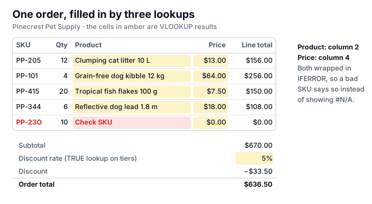
The product name is the same formula with column 2: =VLOOKUP(B2, Products!$A$2:$E$11, 2, FALSE). The line total is plain arithmetic, =C2*E2. Four lines price correctly: $156.00, $256.00, $150.00 and $108.00, a subtotal of $670.00.

The fifth line shows #N/A. Someone typed PP-23O with a capital letter O where the zero should be, and no SKU on the list matches. That error is VLOOKUP doing its job. The next section shows what happens when you don't let it.

VLOOKUP exact match vs approximate match: FALSE or TRUE

The last argument changes how VLOOKUP searches, not just how strict it is.

• FALSE (or 0) checks every row from the top and stops at the first value that matches exactly. If nothing matches, you get #N/A. Order doesn't matter.
• TRUE (or 1, or nothing) assumes the first column is sorted smallest to largest and returns the largest value that is less than or equal to what you asked for. Microsoft's reference says to sort the first column before using it this way. It never tells you it settled for a near miss.

Here's what that means for the PP-23O typo. With FALSE it's #N/A, and someone fixes the SKU. With TRUE, VLOOKUP looks for the last SKU that sorts at or before PP-23O. Digits sort before letters, so PP-230 qualifies, and the formula quietly prices ten bags of cat litter at $4.50, the price of a pack of salmon cat treats.

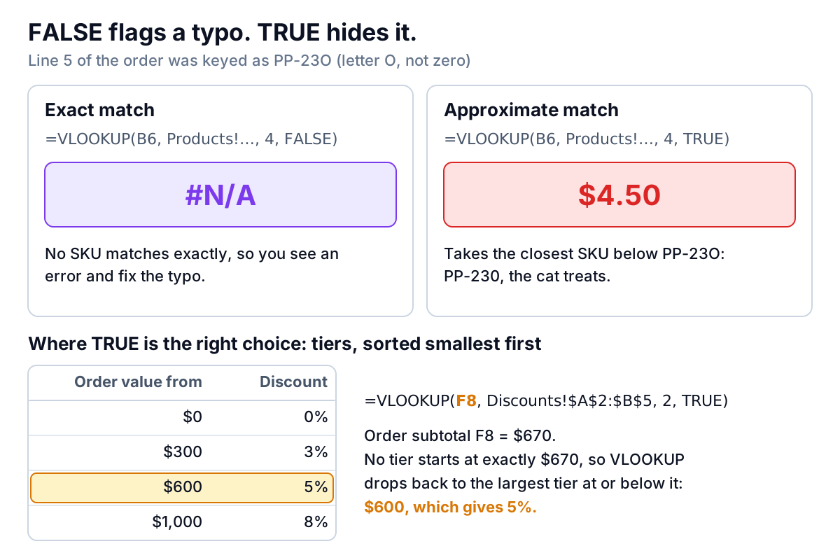
Approximate match does have a proper job: any table of bands, where a value falls between two thresholds. Pinecrest gives trade customers a discount by order value: 0% from $0, 3% from $300, 5% from $600 and 8% from $1,000. With the tiers sorted smallest first on a Discounts sheet, =VLOOKUP(F8, Discounts!$A$2:$B$5, 2, TRUE) returns 5% for the $670 subtotal, because $600 is the largest threshold at or below $670. The discount is $33.50 and the order total $636.50. Shipping bands, commission tiers, tax brackets and age bands for overdue invoices all work the same way.

Column numbers, and how to stop them breaking

The column number is a plain count, so it doesn't know what's in the column. If someone inserts a "Supplier" column between unit cost and price on the Products sheet, price becomes the 5th column, your formulas keep returning column 4, and the order fills with unit costs instead of selling prices. There's no error to warn you.

Three ways to protect yourself:

• Find the column by its header. Replace the 4 with MATCH("Price", Products!$A$1:$E$1, 0), which returns the position of the "Price" heading. The full formula is =VLOOKUP(B2, Products!$A$2:$E$11, MATCH("Price", Products!$A$1:$E$1, 0), FALSE). Insert a column and MATCH counts again. Row 15 of the Solution sheet has it.
• Turn the price list into a table (Insert > Table). VLOOKUP can then point at the table's name, and Microsoft's notes on structured references explain how the reference grows as you add rows, so new products are picked up without editing the formula.
• Use XLOOKUP if everyone has it. It takes the return column as a range rather than a number. It's in Excel for Microsoft 365, Excel 2021 and later, but not in Excel 2016 or 2019. Our XLOOKUP guide covers it.

One more limit comes from the same design: VLOOKUP can only return columns to the right of the lookup column. If you have the product name and need the SKU, which sits to its left, VLOOKUP can't do it. Use INDEX with MATCH, or XLOOKUP.

Catching errors with IFERROR and IFNA

A column of #N/A breaks any total that adds it up, and it looks alarming in a report. Wrap the lookup so it says something useful instead:

=IFERROR(VLOOKUP(B2, Products!$A$2:$E$11, 2, FALSE), "Check SKU")
=IFERROR(VLOOKUP(B2, Products!$A$2:$E$11, 4, FALSE), 0)

Pinecrest's order now shows "Check SKU" against the typo and a price of $0, so the subtotal still adds up to $670.00 while the bad line stands out. Use a word for text columns and 0 for number columns that feed totals.

There's a catch. IFERROR hides every error type, including #REF! from a wrong column number and #NAME? from a typo in the function name. If you'd rather hide only "not found", use IFNA instead: =IFNA(VLOOKUP(B2, Products!$A$2:$E$11, 4, FALSE), 0). Anything else still shows, so a broken formula can't pass for a missing product.

Here are the errors you'll meet and what each one usually means, taken from Microsoft's reference:

If your formula is set up right and still fails, our VLOOKUP not working guide takes each cause in turn, including the invisible characters that come in with exported data, and the Microsoft #N/A guide has more.

Things VLOOKUP won't do on its own

• Return more than the first match. If a SKU appears twice, VLOOKUP returns the first row every time. Price lists that keep old prices further up give old prices.
• Match on two things at once, such as product and size. You need a helper column or an array formula; see VLOOKUP with multiple criteria.
• Look in a different file without care. It can, but the reference changes and links can break when files move. VLOOKUP from another sheet covers other sheets, other workbooks and what breaks them.
• Behave identically in Google Sheets. Mostly it does, but whole-column formulas and links to other files work differently; see VLOOKUP in Google Sheets.

It can, though, use wildcards. With FALSE and a text lookup value, ? matches any single character and * any run of characters, so =VLOOKUP("Salmon*", Products!$B$2:$D$11, 3, FALSE) returns the price of the first product whose name starts with "Salmon". To search for a real asterisk or question mark, put a tilde (~) in front of it.

A checklist before you trust a VLOOKUP column

1. The last argument says FALSE, unless this is a threshold table sorted smallest first.
2. The table range has dollar signs, or points at a table.
3. The column number is right, or it comes from MATCH.
4. Count the #N/A results before you hide them: =COUNTIF(D2:D6, "Check SKU") tells you how many lines need a look.
5. Spot-check one row by hand against the source list.
6. The lookup column has no duplicates. =COUNTIF(Products!$A$2:$A$11, A2) next to each SKU should show 1.

Lookups like this are often the first step in a monthly job: matching an order export to a price list or cost sheet so you can see margin by product, then building an inventory dashboard or an Excel dashboard on top. If you're redoing those lookups every month to join exports from your shop and your accounting system, Parity can take the files directly. Upload the order export and the product list (or connect Shopify or QuickBooks Online) and it builds a dashboard with headline numbers, charts and a table of what needs attention, with every number checked against queries on the full dataset before you see it. You can export the result to Excel, and update it with next month's file.

When you do write VLOOKUPs by hand, the workbook above is a good place to practise: try deleting the FALSE on line 5, insert a column in the price list, and watch what each change does to the order total before it happens in a file that matters.