To use XLOOKUP, type =XLOOKUP(what to find, where to look, what to return): for example =XLOOKUP(H2,A2:A11,D2:D11) finds the SKU in H2 in column A and returns its price from column D. It matches exactly unless you tell it otherwise, returns #N/A when nothing matches (or your own message, if you add a fourth argument), and works in Microsoft 365, Excel 2021 and Excel 2024, but not in Excel 2016 or 2019.
That covers most days. The other three arguments are where XLOOKUP earns its place: discount tiers, partial names, the latest price in a log, several columns from one formula. This guide walks through each one on a single example business, Harlow Hardware, a fictional hardware store with ten products, a discount table, a supplier cost log and one contractor order. Every formula below is in the workbook, with a Practice sheet to try it and a Solution sheet to check yourself.
Download the practice workbook (.xlsx)
The XLOOKUP formula in one picture
Harlow's product list sits in A1:E11: SKU, item, category, unit price and stock on hand. The counter staff type a SKU in H2 and want the price in I2.
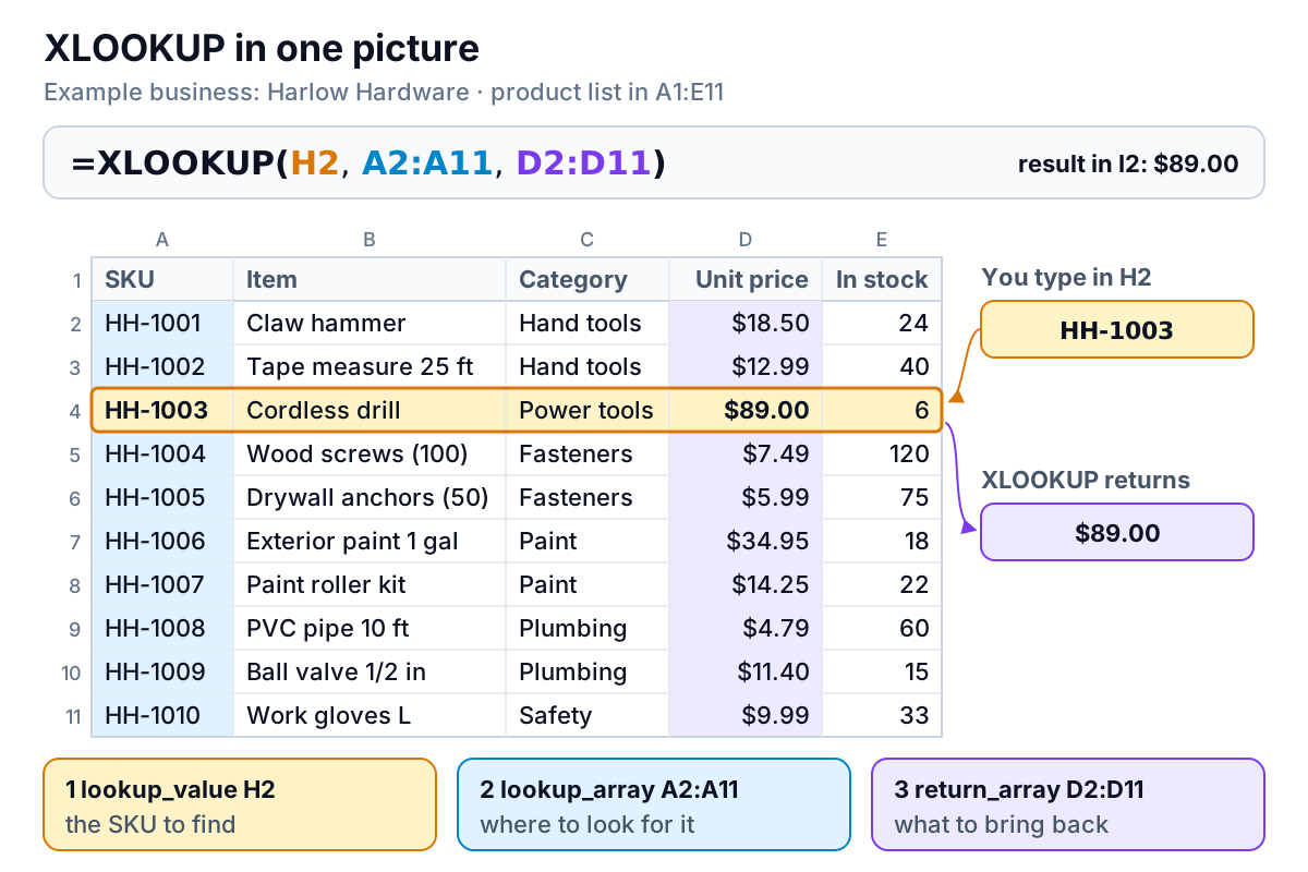
Read the formula left to right as a sentence: "find H2 in A2:A11 and give me the matching item from D2:D11." With HH-1003 in H2, XLOOKUP walks down column A, stops at row 4, and returns the value from row 4 of column D: $89.00, the cordless drill.
Two rules make this work. First, the lookup range and the return range must be the same height. Column A runs from row 2 to row 11, so the return range must too; if one is A2:A11 and the other D2:D10, Excel returns #VALUE! (Exceljet's reference covers this and other edge cases). Second, the return range can be anywhere. It can sit to the left of the lookup column, on another sheet, or be several columns wide. That's the big change from VLOOKUP, which counts columns to the right of the first one. The full side-by-side is in our XLOOKUP vs VLOOKUP comparison.
Want a SKU from an item name instead? Swap the ranges: =XLOOKUP("Paint roller kit",B2:B11,A2:A11) returns HH-1007, even though the SKU column is to the left.
Every XLOOKUP argument, and when you need it
Here is the full syntax from Microsoft's XLOOKUP reference, with the defaults Excel uses when you leave an argument out:
=XLOOKUP(lookup_value, lookup_array, return_array, [if_not_found], [match_mode], [search_mode])
| Argument | What it does | Default | Use it when |
|---|---|---|---|
lookup_value | The value to find | Required | Always. Usually a cell reference |
lookup_array | The single row or column to search | Required | Always |
return_array | The range to return from, same height (or width) as lookup_array | Required | Always. Make it wider to return several columns |
if_not_found | What to show when there's no match | #N/A | A friendly message, a 0 or a blank |
match_mode | 0 exact, -1 exact or next smaller, 1 exact or next larger, 2 wildcard | 0 | Tiers, bands, partial names |
search_mode | 1 first to last, -1 last to first, 2 or -2 binary search on sorted data | 1 | The latest entry in a log |
To skip an optional argument, leave a gap between the commas. =XLOOKUP(H6,A15:A18,B15:B18,,-1) leaves if_not_found empty and sets match_mode to -1.
if_not_found: say what went wrong
If someone types HH-1050, which doesn't exist, the plain formula returns #N/A. Add a fourth argument and it returns your text instead: =XLOOKUP(H3,A2:A11,D2:D11,"Check SKU"). Use words that tell the reader what to do. "Check SKU" is better than "Error", and much better than a 0, which can quietly flow into a total as if the item were free.
match_mode: what happens between the values
Harlow gives contractors a discount by order size: 5% from $250, 8% from $500 and 10% from $1,000. The tiers sit in A15:B18, listed by their lower edge (0, 250, 500, 1,000). A contractor's order comes to $609.49. There's no row for exactly 609.49, so the exact-match default returns #N/A. match_mode tells XLOOKUP which way to go instead.
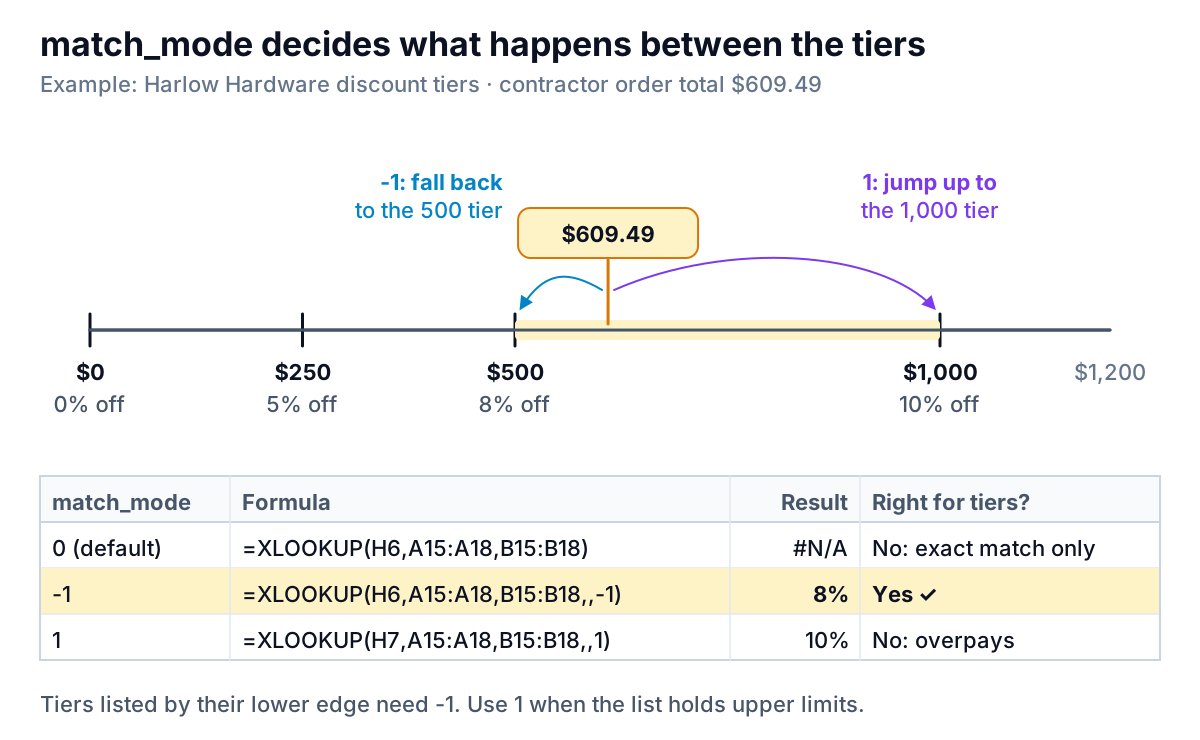
- -1 (exact or next smaller):
=XLOOKUP(H6,A15:A18,B15:B18,,-1)returns 8%, because 500 is the largest tier at or below 609.49. That's correct. - 1 (exact or next larger): the same formula with
,,1)returns 10%, from the 1,000 tier. That's wrong here; 1 is for tables listed by their upper limit, such as "up to 5 kg". - 2 (wildcard): turns on
*(any characters),?(one character) and~(treat the next character literally).=XLOOKUP("*"&H8&"*",B2:B11,D2:D11,"No match",2)with "gloves" in H8 returns $9.99 for "Work gloves L". Without the 2, the asterisks are treated as text and you get#N/A. Microsoft's wildcard guide lists the three characters.
Unlike VLOOKUP's approximate match, XLOOKUP's -1 and 1 don't need the tier table sorted. Keep it sorted anyway, so a person can read it.
search_mode: which match wins
XLOOKUP returns the first match it finds. That's fine for a product list where each SKU appears once. It's a problem in a log, where the same SKU appears every time a supplier invoice comes in. Harlow's cost history in A21:C29 has three rows for the exterior paint, HH-1006, in date order.
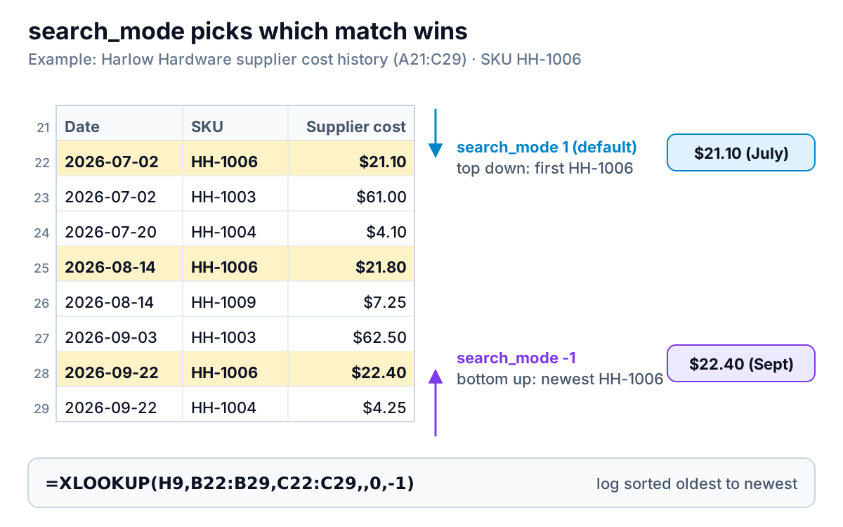
=XLOOKUP(H10,B22:B29,C22:C29) returns $21.10, the July cost, because it reads from the top. =XLOOKUP(H9,B22:B29,C22:C29,,0,-1) reads from the bottom and returns $22.40, the September cost. If you price from the latest cost, the first version understates it by $1.30 a gallon. Reverse search only gives "latest" if the log is in date order, oldest at the top, which is how most exports arrive.
The binary modes, 2 and -2, are for very large lists sorted ascending or descending. They're faster, but Microsoft warns that unsorted data gives invalid results, with no error to tell you. For a list of a few thousand rows, leave search_mode at 1 or -1.
Return several columns with one XLOOKUP
Make the return range wider and XLOOKUP returns the whole slice of the row. =XLOOKUP(H5,A2:A11,B2:E11) in I5, with HH-1006 in H5, fills I5:L5 with the item, category, price and stock: Exterior paint 1 gal, Paint, $34.95, 18.
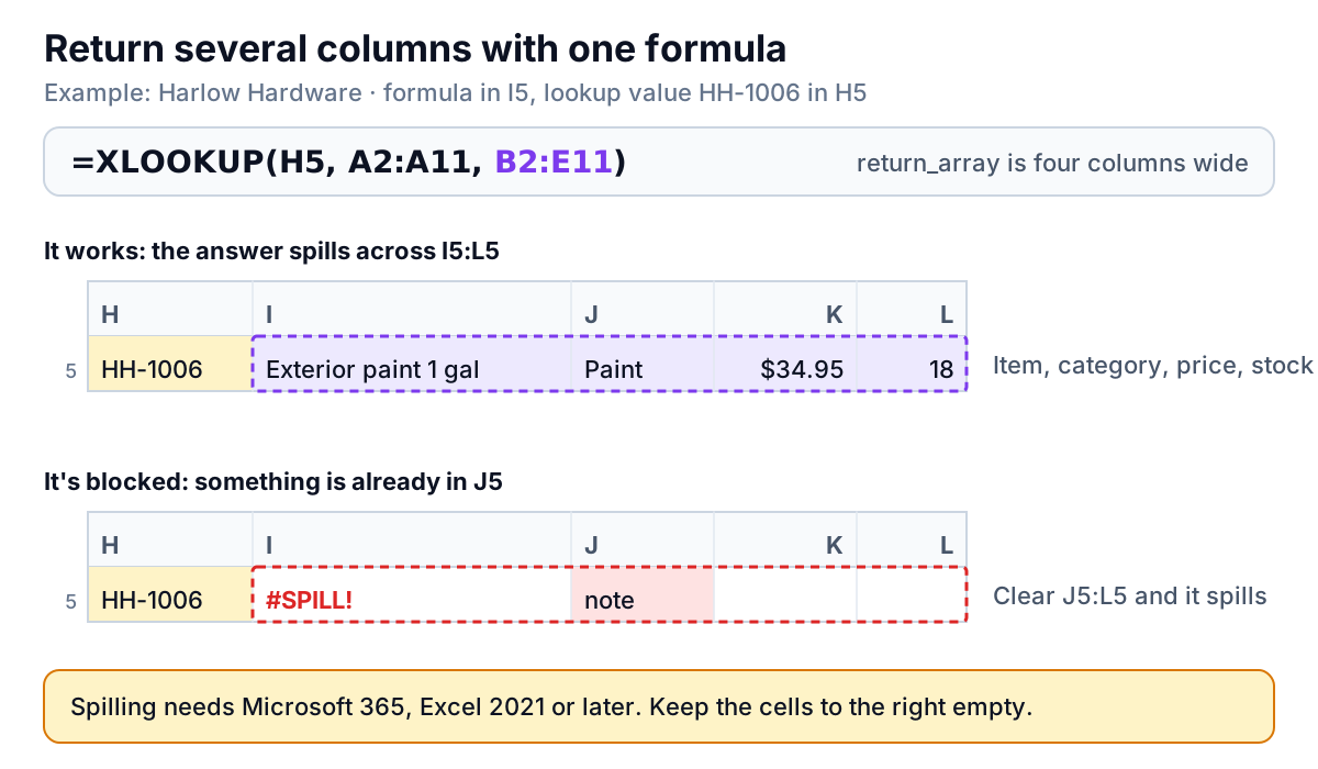
Excel calls this spilling. It needs the cells the answer will fill to be empty; if J5 holds a note, I5 shows #SPILL!. Select the error cell and Excel outlines the range it wanted, and its #SPILL! guide shows how to jump to the cell in the way. You only type the formula in I5; the other cells show the spilled values and can't be edited on their own. Microsoft's page on dynamic arrays and spilling covers the rules.
Worked example: pricing a contractor order
Here's how the pieces fit on a real task. A contractor's order lands as five SKUs and quantities in A33:B37. Harlow needs a price per line, a subtotal and the discount.
In C33, look up the unit price with the ranges locked by dollar signs, then copy it down to C37:
=XLOOKUP(A33,$A$2:$A$11,$D$2:$D$11)
=B33*C33in D33 for the line total
Without the dollar signs, copying down shifts the ranges to A3:A12, then A4:A13, and the lookups start missing the top of the list. This is the most common reason a column of lookups works in the first row and fails lower down.
| SKU | Item | Qty | Unit price | Line total |
|---|---|---|---|---|
| HH-1003 | Cordless drill | 2 | $89.00 | $178.00 |
| HH-1006 | Exterior paint 1 gal | 8 | $34.95 | $279.60 |
| HH-1007 | Paint roller kit | 4 | $14.25 | $57.00 |
| HH-1004 | Wood screws (100) | 6 | $7.49 | $44.94 |
| HH-1010 | Work gloves L | 5 | $9.99 | $49.95 |
| Subtotal | $609.49 | |||
| Discount | 8% tier | −$48.76 | ||
| Order total | $560.73 |
The discount rate in C39 is =XLOOKUP(D38,$A$15:$A$18,$B$15:$B$18,,-1), the tier lookup from earlier pointed at the subtotal. Check the arithmetic: $609.49 × 8% = $48.76 after rounding, and $609.49 − $48.76 = $560.73. If the contractor adds another $390.51 of stock, the subtotal reaches $1,000 and the same formula moves them to 10% without anyone editing it.
XLOOKUP errors and how to fix each one
Most broken lookups come down to a handful of causes. Work down this table in order; the first two cover most cases.
| What you see | Likely cause | Fix |
|---|---|---|
#N/A for a value you can see in the list | A hidden space: "HH-1004 " pasted from an export isn't "HH-1004" | Wrap the value in TRIM: =XLOOKUP(TRIM(H11),A2:A11,D2:D11), or clean the column once |
#N/A for numeric codes | Text vs number: 40112 typed as a number, stored as text in the list (or the reverse) | Convert the column to numbers, or match the type in the formula: TEXT(H2,"0") or VALUE(H2) |
#N/A for a partial name | Wildcards without match_mode 2 | Add ,,2 or ,"No match",2 at the end |
#N/A for an amount between tiers | Exact match on a banded table | Use match_mode -1 (tiers by lower edge) or 1 (by upper limit) |
#VALUE! | lookup_array and return_array are different sizes | Make both cover the same rows, such as A2:A11 and D2:D11 |
#SPILL! | Cells the result needs aren't empty | Clear the cells to the right (or below) |
#NAME? | Typo in the function name, or a version without XLOOKUP | Check spelling; see versions below |
| A wrong value, no error | Binary search on unsorted data, wrong match_mode direction, ranges that moved when copied, or duplicates where you wanted the latest | Use search_mode 1 or -1, check the tier direction, add $ signs, use -1 for logs |
If you'd rather show a blank than an error on a printed report, use if_not_found with "". Avoid wrapping XLOOKUP in IFERROR: it also hides the #VALUE! and #SPILL! errors that point at a real problem.
Which Excel versions have XLOOKUP
XLOOKUP is in Excel for Microsoft 365 (Windows, Mac and the mobile apps), Excel 2021 and Excel 2024. Microsoft's reference says plainly that it is not available in Excel 2016 and Excel 2019, even though those versions can open a file that contains it. In those versions the formula can't calculate and shows #NAME?, Excel's error for a name it doesn't recognise; often you'll also see an _xlfn. prefix in front of the function name.
So before you send a workbook to a client, a bookkeeper or a supplier, ask what they open it in. If anyone is on Excel 2019 or older, use INDEX and MATCH for that file; our XLOOKUP vs INDEX MATCH guide covers the trade-offs and the formulas that work everywhere. Google Sheets has its own XLOOKUP with the same six arguments, so a file shared through Sheets will usually keep working.
One more variation comes up often: looking up on two or three conditions at once, such as style, size and colour. That needs a slightly different pattern, covered step by step in XLOOKUP with multiple criteria.
When the lookup is only step one
For Harlow, XLOOKUP is how a sales export, a price list and a supplier log get joined so someone can answer a question: which products sell at the thinnest margin, what's running low, what changed since last month. If you're rebuilding that join every month from a QuickBooks or Shopify export, the lookups are the part most likely to break, usually because a column moved or a code arrived with a trailing space.
Parity can do that step from the files themselves. Upload the exports (CSV or Excel), or connect QuickBooks Online or Shopify directly, and it builds a dashboard with the headline numbers, charts, what explains them, and a table of what needs attention, such as items below their reorder level. Every number is checked against queries on the full dataset before you see it, and you can export the result to Excel if you want to keep working on it. For the stock side specifically, our inventory dashboard guide shows what to put on the page.
Upload your sales and stock exports and get a checked dashboard without stitching the files together with XLOOKUP first. Build a report from your data free
If you remember one thing, make it the three-part sentence: find this, in here, and bring back that. Everything else is a dial on top of it, and each dial is a small number at the end of the same XLOOKUP formula.