To use XLOOKUP with multiple criteria, multiply the conditions and look for a 1: =XLOOKUP(1,(A2:A13=I2)*(B2:B13=J2)*(C2:C13=K2),E2:E13) returns the value from column E on the first row where all three columns match. The other common way is to join the conditions into one key, =XLOOKUP(I4&"|"&J4&"|"&K4,A2:A13&"|"&B2:B13&"|"&C2:C13,E2:E13), which gives the same answer as long as you keep the separator.
Either XLOOKUP multiple criteria method needs Microsoft 365, Excel 2021 or Excel 2024. This guide uses Kingfisher Uniforms, a fictional workwear supplier whose stock list has a row for every style, size and colour, and shows why the two methods work, the mistakes that return a wrong answer with no error, and what to do when the sheet gets big. Every formula is in the practice workbook, with a Practice sheet to try and a Solution sheet to check.
Download the practice workbook (.xlsx)
Why one condition isn't enough
Kingfisher's list in A1:E13 has 12 rows: style, size, colour, unit price and stock. A café orders navy polos in size L, and the person taking the call checks stock. "Polo" appears six times, and "Polo, L" twice: once in black, with none in stock, and once in navy, with 32.
If you only match on what seems unique, XLOOKUP still gives an answer, just not the right one. A two-condition formula, =XLOOKUP(1,(A2:A13=I3)*(B2:B13=J3),E2:E13), returns 0, because the black polo in row 4 comes before the navy one and XLOOKUP returns the first match. The café is told the polos are out of stock when there are 32 on the shelf.
That's the rule to start from: your conditions must pin down exactly one row. A quick way to check is to count the matches with COUNTIFS before you trust the lookup. =COUNTIFS(A2:A13,"Polo",B2:B13,"L") returns 2, so style and size aren't enough; add colour and it returns 1.
Method 1: multiply the conditions
This is the method to learn first, because it handles any kind of condition, not just "equals".
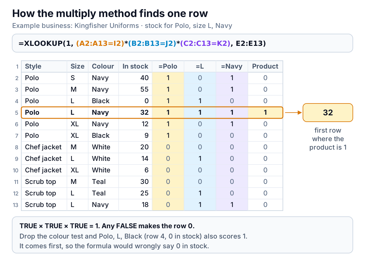
=XLOOKUP(1,(A2:A13=I2)*(B2:B13=J2)*(C2:C13=K2),E2:E13,"No match")
Here's what Excel does with it, step by step:
(A2:A13=I2)compares every style with "Polo" and produces 12 TRUE/FALSE values. The size and colour tests do the same.- Multiplying turns TRUE into 1 and FALSE into 0. A row only scores 1 if it scores 1 on every test, because anything times 0 is 0.
- That list of twelve 1s and 0s becomes the lookup array. XLOOKUP searches it for the value 1 and returns the matching row from E2:E13: 32.
Microsoft uses the same multiply trick in its FILTER function examples for "multiple criteria", so it's well-trodden ground. Return two columns, D2:E13, and you get price and stock together: for a white chef jacket in XL, =XLOOKUP(1,(A2:A13=I5)*(B2:B13=J5)*(C2:C13=K5),D2:E13) spills $36.00 and 6 into two cells.
Conditions that aren't "equals"
Because each condition is just a comparison, you can use any of them. Kingfisher wants the first polo colour in size XL with at least 10 in stock:
=XLOOKUP(1,(A2:A13=I6)*(B2:B13=J6)*(E2:E13>=K6),C2:C13,"None in stock")
With 10 in K6 it returns Navy (12 in stock; the black XL has 9). Raise K6 to 13 and it returns "None in stock". The same pattern takes dates ((D2:D500>=DATE(2026,9,1))), amounts, or anything else you can compare.
OR conditions: add instead of multiply
Multiplying means AND. Adding means OR. To find the first polo in size L that is black or navy and actually in stock:
=XLOOKUP(1,(A2:A13=I7)*(B2:B13=J7)*(((C2:C13="Black")+(C2:C13="Navy"))>0)*(E2:E13>0),C2:C13,"None in stock")
It returns Navy, because the black row fails the stock test. The >0 around the OR part matters when both alternatives can be true on the same row: two TRUEs add up to 2, and XLOOKUP is looking for exactly 1. Wrapping it in >0 turns any positive sum back into a clean TRUE.
(A2:A13="Chef*") looks for the literal text "Chef*". For a partial match inside the multiply method, use ISNUMBER(SEARCH("chef",A2:A13)) as the condition: =XLOOKUP(1,ISNUMBER(SEARCH("chef",A2:A13))*(B2:B13="XL"),D2:D13) returns $36.00.Method 2: join the conditions into one key
The concatenation method glues each row's columns into one piece of text and looks up your inputs glued the same way:
=XLOOKUP(I4&"|"&J4&"|"&K4,A2:A13&"|"&B2:B13&"|"&C2:C13,E2:E13,"No match")
Row 5 becomes "Polo|L|Navy", your inputs become "Polo|L|Navy", and XLOOKUP finds an ordinary exact match: 32. It's easy to read, and it feels like a normal lookup. It only does "equals", though, and it has one trap.
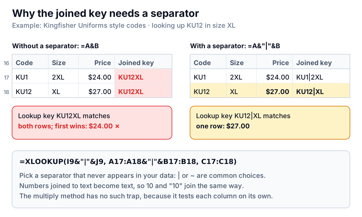
Kingfisher's newer style codes show it. Code KU1 in size 2XL and code KU12 in size XL both join to "KU12XL". Look up KU12 in XL without a separator, =XLOOKUP(I8&J8,A17:A18&B17:B18,C17:C18), and you get $24.00, the KU1 price, with no error. With the pipe, =XLOOKUP(I9&"|"&J9,A17:A18&"|"&B17:B18,C17:C18), the keys are "KU1|2XL" and "KU12|XL" and you get the right $27.00.
Use a separator character that never appears in your data; a pipe or tilde usually works. The multiply method never has this problem, because it tests each column separately.
Choosing between the two methods
Both are correct XLOOKUP multiple criteria formulas when they're written carefully. Pick by the shape of the question:
| Situation | Use | Why |
|---|---|---|
| All conditions are "equals" and you want the simplest formula to read | Join, with a separator | Reads like an ordinary lookup |
| Any condition is a range, a minimum, a date window or an OR | Multiply | Each condition is its own comparison |
| Codes that might run together (KU1 + 2XL) | Multiply, or join with "|" | No key collisions |
| Sizes or codes that are numbers in one place and text in another | Join | Joining turns both into text, so 32 and "32" match |
| The same lookup copied down hundreds or thousands of rows | Helper column, then a plain XLOOKUP | The key is built once per row, not once per formula |
If you're unsure, start with the multiply method. It's the one that keeps working when next month's question adds "and only if it's in stock".
XLOOKUP multiple criteria on big sheets: keep it fast
On Kingfisher's 12 rows, either method calculates instantly. On an order sheet with thousands of lines, each looking up a list with thousands of products, it can slow down. Each multiply-method formula builds a fresh array for every condition, the full length of the range, every time the sheet recalculates; the concatenation method builds a joined array of the same length. Repeat that across every order line and the work adds up.
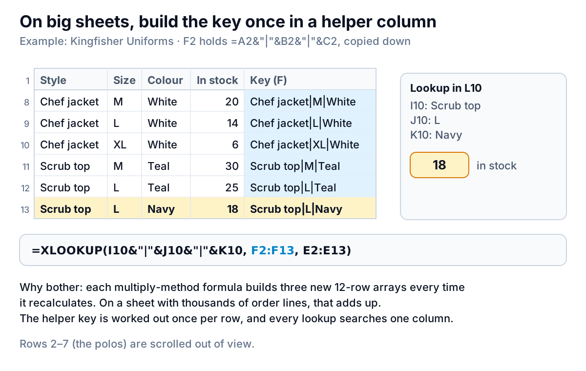
Three habits keep it fast:
- Use a helper column for repeated lookups. Put
=A2&"|"&B2&"|"&C2in F2 and copy it down. Then each lookup is=XLOOKUP(I10&"|"&J10&"|"&K10,F2:F13,E2:E13), which searches one existing column instead of building new ones. For Scrub top, L, Navy it returns 18. - Never point the multiply method at whole columns.
A:Ais over a million rows (Excel's limit is 1,048,576 rows per sheet), and every condition would compare all of them. Use the real range, or format the list as a Table so the range grows with it. - Keep the multiply method for one-off answers. A summary cell or a dashboard input is fine. Two thousand copies of it down an order sheet is where the helper column pays off.
Errors and silent mistakes, and how to fix them
| What you see | Likely cause | Fix |
|---|---|---|
#N/A when the row clearly exists | A typo or a trailing space in one condition ("Navy " vs "Navy"), or one condition that matches nothing | Test each condition alone with COUNTIF; wrap inputs in TRIM |
#N/A on sizes or codes like 10 or 32 | Text vs number: 32 typed as a number, stored as text in the list | Convert the column, or compare like with like. The join method avoids this, because joining turns everything into text |
#VALUE! | The condition ranges or the return range cover different rows (A2:A13 vs B2:B14) | Make every range span the same rows |
| A wrong answer, no error | Conditions that match more than one row, or a joined key without a separator | Check with COUNTIFS; add the missing condition; add "|" |
#SPILL! | Returning several columns into cells that aren't empty | Clear the cells to the right |
#NAME? | Excel 2019 or earlier, which don't have XLOOKUP | Use the INDEX/MATCH version below, or open the file in Microsoft 365 |
When to use FILTER or INDEX/MATCH instead
You want every match, not the first. XLOOKUP always returns one row. To list every colour Kingfisher stocks for a polo in size L, use FILTER with the same conditions: =FILTER(C2:C13,(A2:A13=I12)*(B2:B13=J12),"None") returns Black and Navy as a spilled list, and TEXTJOIN(", ",TRUE,...) around it puts them in one cell. Like XLOOKUP, FILTER needs a recent Excel.
The file has to work in older Excel. INDEX/MATCH does the same multiply trick and works in every version, entered with Ctrl+Shift+Enter in Excel 2019 and earlier:
=INDEX(E2:E13,MATCH(1,(A2:A13=I2)*(B2:B13=J2)*(C2:C13=K2),0))
The 0 at the end of MATCH matters; without it, MATCH assumes sorted data. Our XLOOKUP vs INDEX MATCH guide explains that trap and when INDEX/MATCH is the better choice. If you're still on VLOOKUP, the helper-column key works there too, and XLOOKUP vs VLOOKUP covers when to switch. For the single-condition basics (match modes, the newest entry in a log, spilled results) see the main XLOOKUP guide.
When the lookup feeds a report
For a business like Kingfisher, an XLOOKUP multiple criteria lookup is usually one step in a bigger job: joining order lines to a price or stock list so someone can see what's selling, what's low and what each customer is worth. If you rebuild that join from exports every month, the silent mistakes above are a real risk.
Parity can build that view from the files directly. Upload your order export and stock list (CSV or Excel), or connect Shopify, Square or QuickBooks Online, and it builds a dashboard with the headline numbers and trends, charts, what explains them and a table of what needs attention, such as sizes running low. Every number is checked against queries on the full dataset before you see it. Our inventory dashboard guide shows what's worth tracking.
Upload your orders and stock list and get a checked dashboard, without building multi-condition lookups first. Build a report from your data free
Whichever method you use, run the COUNTIFS check once. If your conditions match exactly one row, both methods give the right answer; if they match two, neither will tell you.