Use XLOOKUP when everyone who opens the file has Microsoft 365, Excel 2021 or Excel 2024: it matches exactly by default, can return a column to the left of the one you search, and keeps working when someone inserts a column. Use VLOOKUP when the workbook will be opened in Excel 2019 or older, because XLOOKUP isn't available there and the formula shows #NAME? instead of an answer.
That's the short answer to XLOOKUP vs VLOOKUP. The longer one matters because VLOOKUP doesn't usually fail loudly. It returns a plausible number that happens to be wrong. To show where, we ran the same lookups both ways on one price list from Hollis Paper Co., a fictional paper and packaging wholesaler with eight SKUs. Both formulas sit next to each other in the practice workbook, so you can change an input and watch them disagree.
Download the practice workbook (.xlsx)
XLOOKUP vs VLOOKUP at a glance
| VLOOKUP | XLOOKUP | |
|---|---|---|
| Syntax | =VLOOKUP(value, table, column_number, [range_lookup]) | =XLOOKUP(value, lookup_range, return_range, [if_not_found], [match_mode], [search_mode]) |
| Default match | Approximate (TRUE) if you leave the last argument out | Exact |
| Return a column to the left | No, only to the right of the first column | Yes, any direction |
| Inserting or deleting a column | Column number doesn't update; can return the wrong column | References move with the data |
| Not found | #N/A; wrap in IFNA for a message | Built-in fourth argument |
| Last match (newest entry) | No | Yes, search_mode -1 |
| Several columns at once | One formula per column in older versions | Yes, one formula spills across |
| Versions | Every Excel version, and Google Sheets | Microsoft 365, Excel 2021, Excel 2024; Google Sheets |
The syntax and defaults come from Microsoft's VLOOKUP and XLOOKUP reference pages. The VLOOKUP page itself now opens with a tip pointing readers to XLOOKUP, which tells you where Microsoft stands.
The same comparison applies sideways. HLOOKUP is VLOOKUP for tables laid out in rows, with a row number instead of a column number, and it has the same approximate-match default and the same habit of breaking when rows are inserted. XLOOKUP covers both directions: point it at a row instead of a column and it works as a horizontal lookup, which Microsoft's HLOOKUP page also suggests. So the XLOOKUP vs VLOOKUP verdict below holds for HLOOKUP too.
The tests below aren't edge cases picked to make VLOOKUP look bad. A mistyped code, a lookup in the "wrong" direction and a column added by a colleague are things that happen in an ordinary month in most small-business spreadsheets.
Five lookups on the same price list
Hollis's price list is in A1:D9: SKU, item, pack size and price, sorted by SKU. Each test types an input in column G, puts a VLOOKUP in column H and an XLOOKUP in column I.
Test 1: a plain price lookup (they agree)
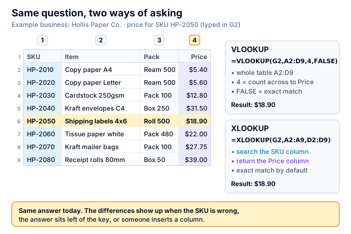
=VLOOKUP(G2,A2:D9,4,FALSE)→ $18.90
=XLOOKUP(G2,A2:A9,D2:D9)→ $18.90
For the everyday case, both work. The difference is in what you have to get right. VLOOKUP needs the whole table, the column's position counted from the left (Price is the 4th), and FALSE for an exact match. XLOOKUP needs the column to search and the column to return. Fewer things to count means fewer things to miscount.
Test 2: a typo in the SKU (VLOOKUP gives a wrong price)
Someone types HP-2045, which doesn't exist, and writes the VLOOKUP the way many people do, without the fourth argument.
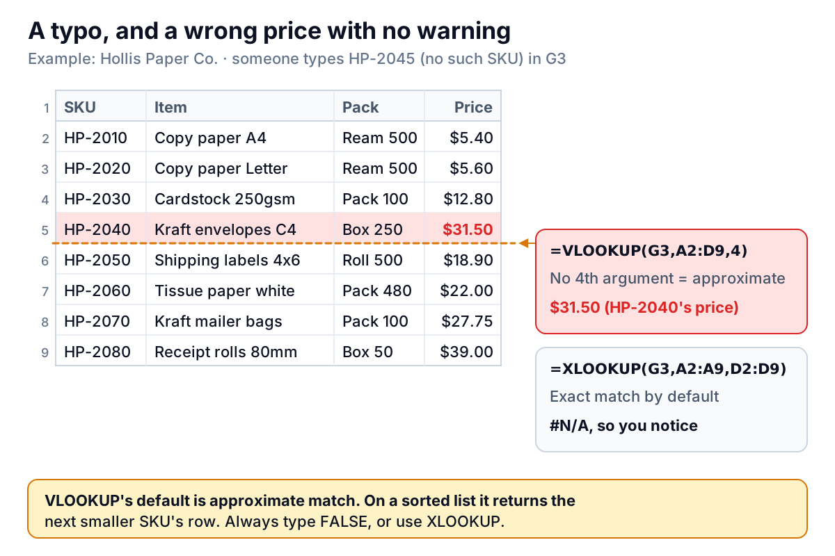
=VLOOKUP(G3,A2:D9,4)→ $31.50
=XLOOKUP(G3,A2:A9,D2:D9)→#N/A
Microsoft's VLOOKUP page is explicit: if you don't specify the last argument, the default is TRUE, approximate match. On a sorted list, approximate match returns the largest value that's smaller than what you asked for, so HP-2045 lands on HP-2040, kraft envelopes at $31.50. Nothing turns red. The order goes out with the wrong price.
XLOOKUP's default is exact, so it returns #N/A, which is the honest answer. To show a message instead, both have a clean option:
=IFNA(VLOOKUP(G4,A2:D9,4,FALSE),"Not found")
=XLOOKUP(G4,A2:A9,D2:D9,"Not found")
Use IFNA rather than IFERROR around VLOOKUP. IFNA only catches "not found"; IFERROR also hides a #REF! from a broken column number, which you want to see.
Test 3: looking to the left
Now the question runs the other way: a customer reads out "Shipping labels 4x6" from an old invoice and you need the SKU. The item is in column B and the SKU in column A, to its left. VLOOKUP always searches the first column of its table and returns something to the right, so it can't do this directly. The usual workaround builds a flipped table with CHOOSE:
=VLOOKUP(G5,CHOOSE({1,2},B2:B9,A2:A9),2,FALSE)→ HP-2050
=XLOOKUP(G5,B2:B9,A2:A9)→ HP-2050
Both return HP-2050. One of them you can read aloud and the other you'll have to explain to whoever opens the file next. The other old fix, moving the SKU column to the right of the item column, changes the layout of a sheet other formulas may depend on.
Test 4: someone inserts a column
A month later, someone adds a Supplier column between Item and Pack. It's a normal thing to do. Excel widens VLOOKUP's table from A:D to A:E automatically, but the column number is just a typed 4, and it stays 4.
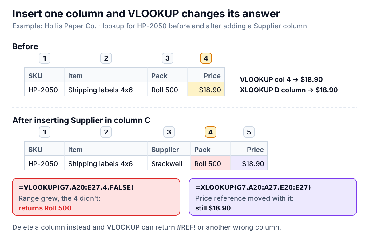
=VLOOKUP(G7,A20:E27,4,FALSE)→ Roll 500
=XLOOKUP(G7,A20:A27,E20:E27)→ $18.90
In this case the error is visible, because "Roll 500" is text where a price should be. If the inserted column had been numeric, say a cost or a reorder level, VLOOKUP would have returned a believable number from the wrong column. Delete a column instead and the table may become narrower than the column number, which gives #REF!. XLOOKUP refers to the price column itself, so inserting or deleting other columns doesn't change which data it returns.
Test 5: shipping bands (they agree again)
Approximate match isn't always a mistake. Hollis charges shipping by weight band: $9 from 0 kg, $14 from 5 kg, $22 from 10 kg and $35 from 20 kg, listed in A13:B16. A 12.5 kg order should pay $22.
=VLOOKUP(G6,A13:B16,2,TRUE)→ $22.00
=XLOOKUP(G6,A13:A16,B13:B16,,-1)→ $22.00
Both are right. The difference is what can go wrong: VLOOKUP's approximate match needs the first column sorted ascending, and Microsoft warns that if it isn't, the result "might be something you don't expect". XLOOKUP's -1 (exact or next smaller) doesn't need sorting. If you keep VLOOKUP for bands, type the TRUE so the next reader knows it was deliberate.
When VLOOKUP still matters
None of this makes VLOOKUP wrong to use. It's still a fully supported function, and in some files it's the better choice:
- Someone opens the file in Excel 2019 or older. Microsoft's XLOOKUP page says it is not available in Excel 2016 and Excel 2019. In those versions an XLOOKUP formula can't calculate and shows
#NAME?. Your accountant, a client or a supplier's buyer may well be on one of them. - You don't control who the file goes to. A price list or quote template that gets forwarded around is safest with functions every version has. VLOOKUP with FALSE, or INDEX/MATCH, works everywhere.
- The workbook already works. A tested VLOOKUP with FALSE, on a table nobody restructures, doesn't need rewriting. Spend the time on the ones without the FALSE.
- Your team reads VLOOKUP fluently. A formula the next person understands beats a cleverer one they don't. That argument fades as people get used to XLOOKUP, but it's real in the meantime.
Google Sheets isn't a reason to avoid XLOOKUP any more: it has its own XLOOKUP with the same arguments. If you need a lookup that works in every Excel version and also looks left, INDEX/MATCH is the classic answer; our XLOOKUP vs INDEX MATCH comparison covers it.
Converting VLOOKUP formulas to XLOOKUP
If you've decided to switch a workbook, the translation is mechanical. Take the first column of the VLOOKUP table as the lookup range, and the column at the given number as the return range:
| VLOOKUP | XLOOKUP | Watch for |
|---|---|---|
=VLOOKUP(G2,A2:D9,4,FALSE) | =XLOOKUP(G2,A2:A9,D2:D9) | Column 4 of A:D is D |
=VLOOKUP(G2,A2:D9,4) or ,TRUE) | =XLOOKUP(G2,A2:A9,D2:D9,,-1) | Decide first: was approximate match intended? For SKUs it almost never is; use exact |
=IFNA(VLOOKUP(...),"Not found") | =XLOOKUP(G2,A2:A9,D2:D9,"Not found") | Drop the wrapper |
=IFERROR(VLOOKUP(...),0) | =XLOOKUP(G2,A2:A9,D2:D9,0) | Ask whether 0 is safe; it can hide a missing price inside a total |
Three checks after converting: the lookup and return ranges cover the same rows (different sizes give #VALUE!), ranges you copy down have their dollar signs, and any VLOOKUP without FALSE gets a deliberate decision rather than a straight copy. That last one often turns up a pricing error that has been sitting there for months. For the full set of XLOOKUP options, including wildcard and newest-entry lookups, see our XLOOKUP guide; for lookups on two or more conditions, such as SKU and customer price band, see XLOOKUP with multiple criteria.
Microsoft has also tuned both functions for speed. Its performance notes say VLOOKUP, HLOOKUP and MATCH got substantial speed improvements, and that XLOOKUP and XMATCH add more for Microsoft 365 users. On a price list of a few hundred rows you won't notice either way; pick on correctness, not speed.
Beyond the lookup
At Hollis, most lookups exist to join two exports: the order lines from the sales system and the price or cost list from the stock sheet, so someone can see margin by product or customer. If that join is a monthly chore, it's also a monthly chance for the errors above to creep in.
Parity takes the exports as they are. Upload the CSV or Excel files, or connect QuickBooks Online or Shopify directly, and it builds a dashboard with headline numbers and their trends, charts, what explains them and a table of what needs attention. Every number is checked against queries on the full dataset before you see it, and you can export the result to Excel. Our sales report guide shows what's worth putting on that page.
Upload your order and price files and get a checked sales dashboard, no VLOOKUP or XLOOKUP to maintain. Build a report from your data free
Whichever function you choose, the one habit that prevents most damage is the same: make a missing value look missing. With XLOOKUP that's the default; with VLOOKUP it's a FALSE you have to remember every time.