To VLOOKUP from another sheet, put the sheet name and an exclamation mark in front of the range: =VLOOKUP(C2, 'Price list'!$A$2:$D$8, 3, FALSE). The single quotes are needed only because the sheet name has a space, and the easiest way to get it all right is to click the other sheet's tab and select the range while you type the formula.
That's the whole trick for sheets in the same file. Other workbooks, other Google Sheets files and sheet names chosen by a formula each have their own syntax and their own ways of breaking, and that's what most of this guide is about. It uses one example business throughout: Juno Print Shop, a fictional print shop pricing this week's jobs from a price list kept on its own sheet. Download the practice workbook (.xlsx): the Practice sheet has the lookup cells blank, the Solution sheet has them filled in, and two price sheets sit alongside.
How to VLOOKUP from another sheet, step by step
Juno's workbook has a Jobs sheet (job number, client, product code, units) and a Price list sheet with seven products: code in column A, product in B, unit price in C and a one-off setup fee in D. To price each job:
- On the Jobs sheet, click F2 (Unit price) and type
=VLOOKUP(. - Click C2, the product code, and type a comma.
- Click the Price list tab at the bottom of the window. Excel switches sheets but keeps building your formula; the formula bar now shows
'Price list'!. - Select A2:D8 and press F4 to lock it:
'Price list'!$A$2:$D$8. - Type
, 3, FALSE)and press Enter. Excel takes you back to the Jobs sheet with the result in F2: $18.00 for 100 A5 flyers. - Copy down. For the setup fee, use the same formula with column 4. The job total is
=D2*F2+G2: units × unit price + setup fee.
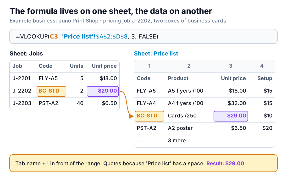
The six jobs come to $901.00. Job J-2202, two lots of 250 business cards, is 2 × $29.00 + $10.00 setup = $68.00. The 40 A2 posters for J-2203 are 40 × $6.50 + $20.00 = $280.00.
Don't skip the F4 step. Without dollar signs, copying the formula down moves the range on the other sheet down with it, which is harder to notice than on the same sheet because you can't see the range move. If prices for products near the top of the list start returning #N/A lower down the job list, that's why. The main VLOOKUP guide covers the other arguments in detail.
Pulling two columns from the other sheet with one formula
Unit price and setup fee come from the same row of the Price list, so you don't need two hand-edited formulas. Juno's Jobs sheet uses the same headings as the Price list ("Unit price" in F1, "Setup fee" in G1), so the column number can come from the heading itself:
=VLOOKUP($C2, 'Price list'!$A$2:$D$8, MATCH(F$1, 'Price list'!$A$1:$D$1, 0), FALSE)Enter it in F2 and copy it right to G2 and down to row 7. The dollar sign before C keeps every copy looking at the product code, and the one before 1 keeps MATCH reading the heading row. For J-2202 it returns $29.00 in F3 and $10.00 in G3. Columns L and M of the Solution sheet show the same formula next to the plain version. This is the sturdiest way to VLOOKUP from another sheet that someone else maintains, because a column added to the Price list moves the heading and MATCH follows it.
Writing the sheet reference by hand
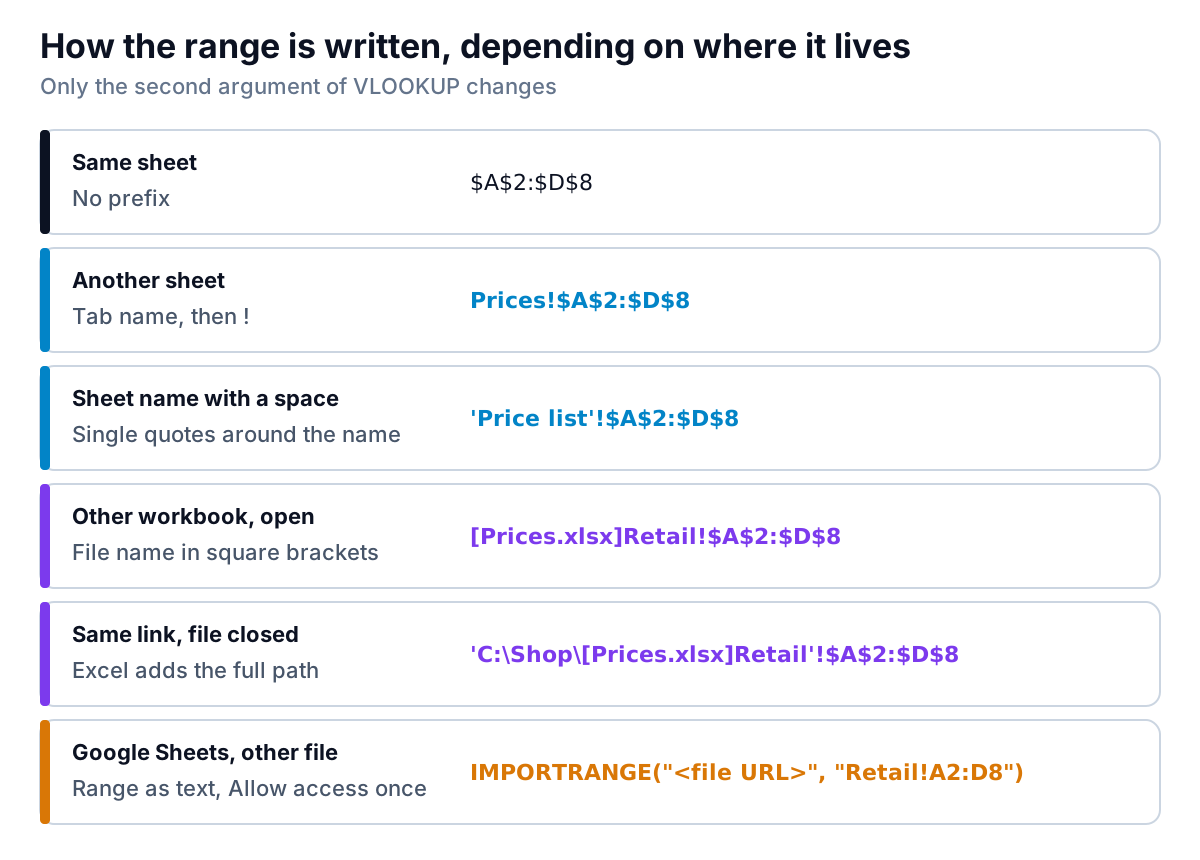
Clicking is safest, but you'll often read or edit these references, so it's worth knowing the rules. Microsoft's guide to external references and Google's guide to referencing other sheets agree on the basics:
- Sheet name, exclamation mark, range:
Prices!$A$2:$D$8. - Single quotes around the sheet name if it contains spaces or other non-alphanumeric characters:
'Price list'!$A$2:$D$8,'Trade prices'!$A$2:$D$8. Quotes around a name that doesn't need them do no harm, so if in doubt, add them. - The quotes go around the sheet name only, and the exclamation mark goes outside them.
VLOOKUP from another workbook
If the price list lives in a separate file, the process is the same: open both files, start the formula in one, switch to the other window and select the range. Excel writes the file name in square brackets in front of the sheet name. Microsoft's examples show the two forms:
- While the source file is open:
[Prices.xlsx]Retail!$A$2:$D$8 - Once it's closed, Excel shows the full path:
'C:\Shop\[Prices.xlsx]Retail'!$A$2:$D$8
The full formula for Juno would be =VLOOKUP(C2, [Prices.xlsx]Retail!$A$2:$D$8, 3, FALSE). In Excel for the web, the path is the file's OneDrive or SharePoint address.
Three things to know before you rely on it:
- Excel treats these links as potentially unsafe. When the file opens, you're asked whether to enable the content and update the links. Until you do, the formulas show the values saved last time.
- The link is to a path. Rename the price list file, move it to another folder or email the jobs file to someone else, and the link can't find its source. Fix it from Data > Queries and Connections > Workbook Links, where Microsoft's workbook links guide describes Change source (point the link at the file's new name or location) and Refresh. Older versions call this Data > Edit Links.
- Break links is permanent. The same guide says breaking a link converts every formula that uses it to its current value, and that it can't be undone in desktop Excel. Save a copy first.
A rule of thumb: if two files are always used together by the same person on the same computer, a link is fine. If the jobs file gets shared, emailed or copied each month, paste the current price list into a sheet inside the jobs file instead. A copy that's a week old but present beats a link that points at someone else's C: drive.
Choosing the sheet with INDIRECT
Juno charges trade customers less, from a second sheet called Trade prices with the same layout. Rather than writing two different formulas, put the name of the price sheet on each job (column I) and let INDIRECT turn that text into a reference:
=VLOOKUP(C2, INDIRECT("'"&I2&"'!$A$2:$D$8"), 3, FALSE)The formula glues together a quote, the sheet name from I2, a closing quote and the range, then INDIRECT reads that string as an address. For the bookshop's 40 posters, I4 says "Trade prices", so the unit price is $5.50 instead of $6.50; for the dental practice's brochures, $38.00 instead of $45.00.
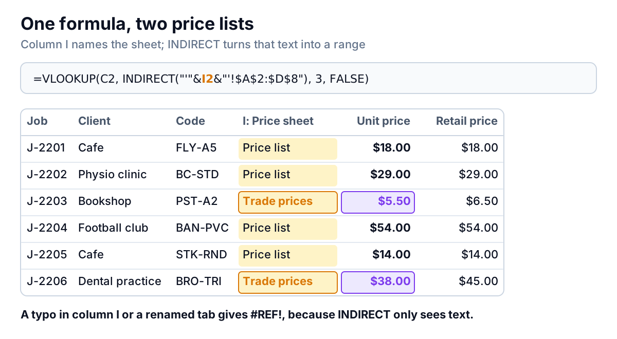
The cost of this flexibility is that Excel no longer knows the formula depends on those sheets. A typo in column I ("Trade price", without the s) gives #REF!. Rename the Trade prices tab and every trade job breaks, because the old name is stored as text. And Microsoft's reference says that if INDIRECT points at another workbook that isn't open, it returns #REF!, so use it only between sheets of the same file. A data validation drop-down in column I that lists the exact sheet names prevents the typos.
Google Sheets: other tabs and other files
Inside one Google Sheets file, the syntax is the same as Excel's: =VLOOKUP(C2, 'Price list'!$A$2:$D$8, 3, FALSE), quotes and all, and clicking the tab while you type works too.
For a different file, Google's help is explicit that you must use IMPORTRANGE, and you can nest it straight inside VLOOKUP:
=VLOOKUP(C2, IMPORTRANGE("https://docs.google.com/spreadsheets/d/…", "'Price list'!A2:D8"), 3, FALSE)The URL and the range are both text in quotation marks. The first time, the cell shows an error until you allow access between the two files; after that, any editor of the jobs file can pull from any part of the price list file. Google caps each import at 10 MB and checks for updates every hour while the file is open. Because the file is identified by its URL, renaming or moving the price list in Drive doesn't break it, which is one advantage over Excel's file-path links. Our VLOOKUP in Google Sheets guide shows how to fill a whole column with one formula.
What breaks a cross-sheet VLOOKUP
| What happens | Same-workbook reference | Link to another workbook | INDIRECT | IMPORTRANGE |
|---|---|---|---|---|
| Price sheet renamed | Formula updates itself | Updates only if both files are open | #REF!: the name is stored as text | Error: the range is stored as text |
| Price sheet deleted | #REF! | #REF! on next update | #REF! | Error |
| Source file renamed or moved | Not affected | Link can't find it; use Change source | Not used across files | Keeps working |
| Source file closed | Not affected | Shows the last saved values | #REF! | Not affected |
| Column inserted in the price list | The range widens or the text range stays put; either way, column 3 may now be a different column. Find the column with MATCH on the header instead of typing 3 | |||
If a cross-sheet formula fails and none of these apply, the cause is usually the data rather than the reference: numbers stored as text, or spaces after codes in one list. Our VLOOKUP not working guide has the full diagnosis.
Keeping lookups to other sheets easy to maintain
- Give the price list a name. In Excel, select A2:D8 and type a name such as
price_listin the Name Box, or turn it into a table.=VLOOKUP(C2, price_list, 3, FALSE)is easier to read, works from any sheet, and doesn't need quotes. - Short sheet names without spaces (Prices, Trade) save typing and quoting.
- Keep one copy of each list. Two sheets with "the price list" on them drift apart within a month.
- Prefer same-file sheets over links between files for anything you send to someone else.
Lookups across sheets are often a sign that one report is being stitched together from several exports: jobs from one system, prices or costs from another, payments from a third. If you're doing that every month to build a sales report or an Excel dashboard, Parity can work from the exports themselves. Upload the CSV or Excel files and it builds a dashboard with headline numbers, charts and a table of what needs attention, checking every number against queries on the full dataset before you see it. You can refine it by chat, export it to Excel, and update it with next month's file.
Upload your job list and price list and get a checked dashboard of jobs, revenue and what needs attention. Build a report from your data free
For a VLOOKUP from another sheet in the same workbook, though, the rule fits on one line: click the other tab while you type the formula, press F4, and end with FALSE.