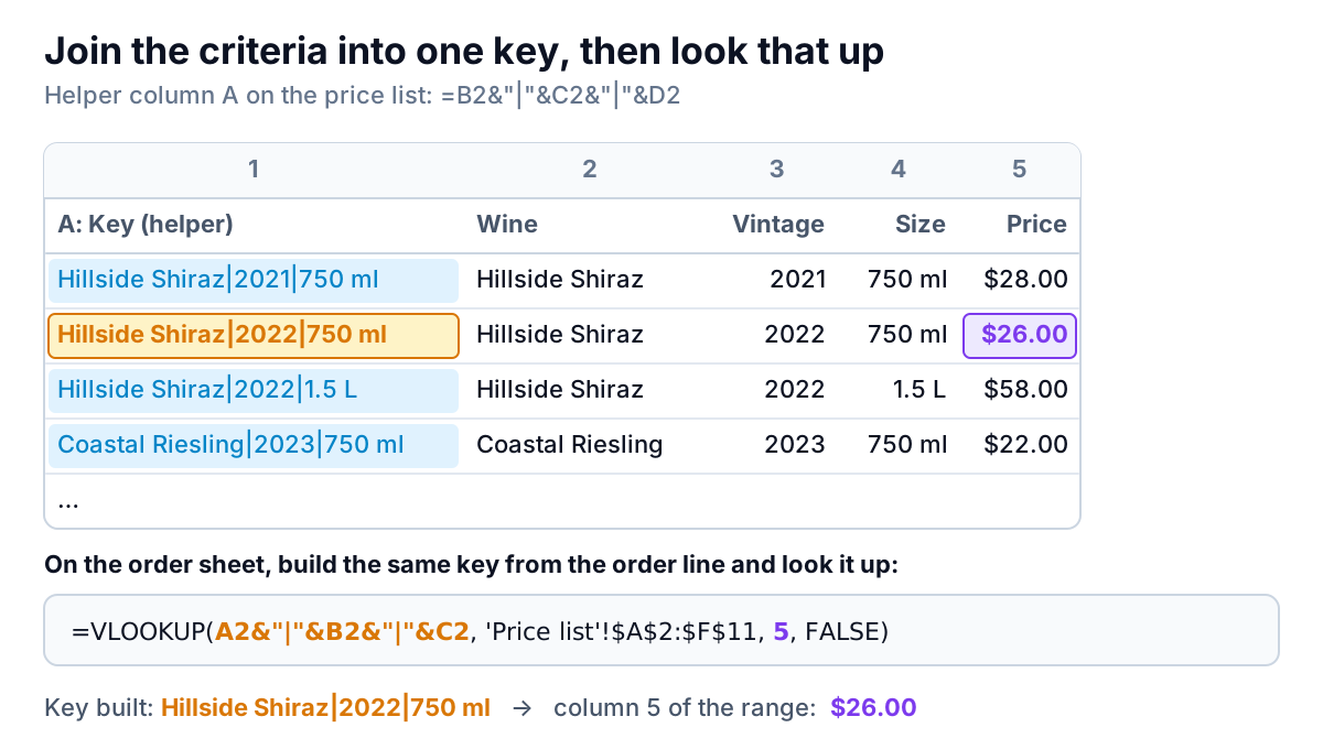
VLOOKUP only matches one value, so to look up on several criteria you join them into one key: add a helper column to the data with =B2&"|"&C2&"|"&D2, then look up the same joined key with =VLOOKUP(A2&"|"&B2&"|"&C2, 'Price list'!$A$2:$F$11, 5, FALSE). If everyone using the file has Microsoft 365 or Excel 2021 or later, XLOOKUP does it without a helper column.
This VLOOKUP multiple criteria guide shows four ways to do it on one example: Redfern Wine Shop, a fictional wine merchant pricing a trade order from a list where the same wine appears in several vintages and bottle sizes. Download the practice workbook (.xlsx). The Practice sheet has the price cells blank; the Solution sheet has every method filled in, plus a column showing what a plain VLOOKUP gets wrong.
Why a plain VLOOKUP picks the wrong row
Redfern's price list has one row per wine, vintage and size. Hillside Shiraz alone has three rows: 2021 in 750 ml at $28, 2022 in 750 ml at $26, and 2022 in a 1.5 L bottle at $58. A restaurant orders a case of the 2022 in 750 ml.
VLOOKUP with an exact match searches the first column from the top and stops at the first match. Microsoft's VLOOKUP reference describes one lookup value in one column, and nothing else gets checked. Look up "Hillside Shiraz" and you get $28, the 2021, every time.
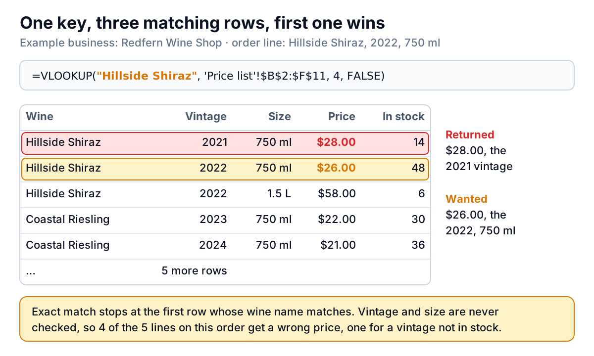
Across the five lines of the example order, the name-only lookup gets four wrong:
| Order line | Qty | Name-only VLOOKUP | Correct price |
|---|---|---|---|
| Hillside Shiraz, 2022, 750 ml | 12 | $28 (the 2021) | $26 |
| Estate Chardonnay, 2023, 375 ml | 24 | $30 (2022, 750 ml) | $16 |
| Old Vine Grenache, 2021, 750 ml | 6 | $34 (the 2020) | $32 |
| Coastal Riesling, 2023, 750 ml | 12 | $22 (right by luck) | $22 |
| Hillside Shiraz, 2020, 750 ml | 6 | $28 | Not on the list |
Priced correctly, the four wines Redfern stocks come to 12 × $26 + 24 × $16 + 6 × $32 + 12 × $22 = $1,152. The name-only version would have charged $28 for a 2020 Shiraz the shop doesn't have, and $30 instead of $16 for half bottles, and the order would have looked perfectly normal.
Method 1: VLOOKUP multiple criteria with a helper column
This is the method to use if you can add a column to the data. It works in every version of Excel and in Google Sheets, it's easy for the next person to read, and it calculates fast.
- Insert a column at the far left of the price list, so it becomes column A. VLOOKUP only searches the first column of the range, so the key has to be there.
- Build the key in A2:
=B2&"|"&C2&"|"&D2, which joins wine, vintage and size intoHillside Shiraz|2022|750 ml. Copy it down. - On the order sheet, build the same key from the order line inside the lookup:
=VLOOKUP(A2&"|"&B2&"|"&C2, 'Price list'!$A$2:$F$11, 5, FALSE). Price is now the 5th column of the range, because the helper pushed everything one to the right. - Handle the missing ones: wrap it as
=IFNA(VLOOKUP(…), "No price"), so the 2020 Shiraz says so instead of showing#N/A.
Why the separator matters
You could join the fields with nothing between them, and most of the time it would work. Then one day two different combinations produce the same text. Bin "RW-1" with shelf "12" and bin "RW-11" with shelf "2" both join to "RW-112", and VLOOKUP will happily return the first. A character that never appears in your data, like a pipe (|), makes every key unique as long as each combination is.
Text and numbers stop being a problem, mostly
Joining with & turns everything into text, so a vintage typed as the number 2022 on one sheet and as the text "2022" on another both become "2022". That removes one of the common reasons a VLOOKUP fails. Two things still bite:
- Trailing spaces. "750 ml " with a space joins to a different key. Clean the source columns with TRIM first; our VLOOKUP not working guide covers spaces you can't see.
- Dates and formatted numbers. A date joins as its underlying serial number, not as it's displayed, and $26.00 joins as 26. If a criterion is a date, join
TEXT(B2,"yyyy-mm-dd")on both sides.
Keeping the helper column up to date
A helper column fails quietly when the list grows and nobody copies the formula down: new wines have no key, so lookups for them return "No price" even though the price is right there. Two habits prevent it:
- Make the price list a table (Insert > Table). A formula typed in the first row of a table column fills the whole column, and Microsoft's notes on structured references explain that references to the table adjust as rows are added, so new wines get a key and the lookup range grows with them.
- Paste new supplier lists into columns B onward only. If you paste over column A, the keys become plain text copied from somewhere else, and they stop updating when a price row changes. A quick test after any paste: the last row of column A should still show a formula, not a value.
You can hide the helper column once it works. Hiding doesn't stop VLOOKUP reading it.
Method 2: no helper column, using CHOOSE
Sometimes you can't change the data: it's a supplier's file, or a report another team overwrites each month. You can build the key column inside the formula instead:
=VLOOKUP(A2&"|"&B2&"|"&C2,CHOOSE({1,2}, 'Price list'!$B$2:$B$11&"|"&'Price list'!$C$2:$C$11&"|"&'Price list'!$D$2:$D$11, 'Price list'!$E$2:$E$11),2, FALSE)
CHOOSE normally picks one value from a list by number. Given the array {1,2}, it returns both choices side by side: a first column of joined keys and a second column of prices. VLOOKUP then searches that two-column table and returns column 2.
This is an array formula. In Microsoft 365 you press Enter as usual. In versions without dynamic arrays, Microsoft's guide to legacy array formulas says to confirm with Ctrl+Shift+Enter, and Excel shows braces around the formula. Forget, and you'll get a wrong result or an error. Columns G and H of the practice workbook are stored as array formulas, so they work in either.
In Google Sheets, build the same table with braces instead of CHOOSE: {ARRAYFORMULA(range1&"|"&range2&"|"&range3), price_range}. Our VLOOKUP in Google Sheets guide explains the array syntax.
The cost is readability. Anyone opening the file later sees a long formula, not a column they can check. On a few thousand rows that's fine; on a large list, the formula rebuilds every key each time the sheet recalculates, so a helper column will feel quicker.
Method 3: INDEX and MATCH with multiplied conditions
If you're writing an array formula anyway, INDEX and MATCH is shorter and has no left-to-right restriction:
=INDEX('Price list'!$E$2:$E$11,MATCH(1, ('Price list'!$B$2:$B$11=A2) * ('Price list'!$C$2:$C$11=B2) * ('Price list'!$D$2:$D$11=C2), 0))
Each comparison in brackets produces a column of TRUE and FALSE. Multiplying them turns TRUE into 1 and FALSE into 0, and a row is 1 only when all three conditions hold. MATCH(1, …, 0) finds the first such row, and INDEX returns the price from it. It needs Ctrl+Shift+Enter in older Excel, like method 2, and returns #N/A when nothing matches.
A nice side effect: unlike the helper key, it compares values directly, so the number 2022 won't match the text "2022". Keep both sides the same type.
When to switch to XLOOKUP or FILTER
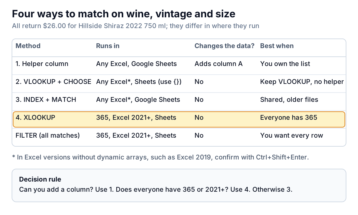
If everyone who opens the file has Excel for Microsoft 365, Excel 2021 or later, or uses Google Sheets, skip VLOOKUP for this job. XLOOKUP takes the same multiplied conditions as its lookup array, needs no special keys, and has a built-in "not found" value:
=XLOOKUP(1, ('Price list'!$B$2:$B$11=A2) * ('Price list'!$C$2:$C$11=B2) * ('Price list'!$D$2:$D$11=C2), 'Price list'!$E$2:$E$11, "No price")Microsoft's page says plainly that XLOOKUP is not available in Excel 2016 and Excel 2019. Anyone on those versions sees #NAME?, which is why VLOOKUP-based methods still matter in shared files. Our XLOOKUP multiple criteria guide goes further.
When you want every match rather than the first, use FILTER (Microsoft 365, Excel 2021 and later, and Google Sheets). To list all bottle sizes of the 2023 Estate Chardonnay with their prices:
=FILTER('Price list'!D2:E11, ('Price list'!B2:B11="Estate Chardonnay") * ('Price list'!C2:C11=2023), "None")That spills two rows: 750 ml at $29 and 375 ml at $16. Multiplying conditions means AND; Microsoft's FILTER page shows adding them with + for OR.
A word on SUMIFS, which some guides suggest for numeric lookups. =SUMIFS(price, wine, A2, vintage, B2, size, C2) does return $26 for a unique combination, in any version, without an array. But it returns 0 when nothing matches (so a missing wine looks free) and adds the prices together if a combination appears twice. Use it only when you've checked each combination is unique, and see our SUMIFS guide for what it's actually built for.
Mistakes that give a wrong price
- Different field order on each side. Wine|vintage|size on the price list and wine|size|vintage in the lookup never match.
- Duplicate combinations. If the 2022 Shiraz 750 ml appears twice, at old and new prices, every method above returns the first. Check with
=COUNTIFS('Price list'!B:B, A2, 'Price list'!C:C, B2, 'Price list'!D:D, C2); anything above 1 needs cleaning. - Range not locked. Without dollar signs, the price list range slides down as you copy, and lower lines miss rows near the top.
- Wrong column number after adding the helper. Price was column 4; with the helper it's column 5.
- A missing
FALSE. On text keys, approximate match returns a neighbouring row's price without any error. The VLOOKUP guide explains why.
Most multi-criteria lookups in a small business exist to join two exports: an order or sales file and a price or cost list, so you can see revenue and margin by product. If you're rebuilding those joins every month to produce a sales report or an inventory dashboard, Parity can take the files directly. Upload the order export and the price list as CSV or Excel and it builds a dashboard of headline numbers, charts and a table of what needs attention, with every number checked against queries on the full dataset before you see it. You can refine it by chat and export it to Excel.
Upload your order export and price list and get a checked sales dashboard by product, vintage or size. Build a report from your data free
If you stay in the spreadsheet, start any VLOOKUP multiple criteria job with the helper column. It's the version you'll still understand in six months, and the COUNTIFS check takes a minute to add.