SUMIFS adds up the numbers in one column for the rows that pass every test you give it: =SUMIFS(sum_range, criteria_range1, criteria1, [criteria_range2, criteria2], …). For example, =SUMIFS(F2:F21, B2:B21, "Harbour Grill", C2:C21, "Prawns") adds the Amount column only where the customer is Harbour Grill and the product is prawns.
The function is in every current version of Excel: Microsoft 365, Excel 2016 through 2024 on Windows and Mac, and Excel for the web, according to Microsoft's SUMIFS reference. The syntax is short. What trips people up is the criteria: how to write "after the 15th", "anything ending in Grill", "not salmon", "blank", or "prawns or snapper". This guide is mostly about those, worked on one month of orders, with the answers you should get.
The example business is Gull Rock Seafood, a fictional wholesale supplier selling to five restaurants, with 20 orders in September 2026 worth $5,807 in total. Download the practice workbook (.xlsx): the Practice sheet has the questions with blank answer cells, and the Solution sheet has every formula.
How SUMIFS reads its arguments
The data sits in A1:G21: order date (A), customer (B), product (C), category (D), kg (E), amount in dollars (F) and paid date (G, blank if unpaid). The first SUMIFS question is how much Harbour Grill spent on prawns.
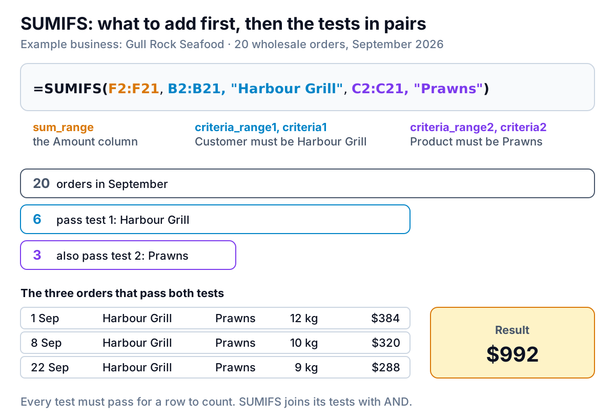
Read it left to right:
- sum_range (F2:F21): the numbers to add. It always comes first in SUMIFS.
- criteria_range1, criteria1 (B2:B21, "Harbour Grill"): the first test. Six orders pass.
- criteria_range2, criteria2 (C2:C21, "Prawns"): the second test. Three of those six pass.
Three rules hold for every SUMIFS formula:
- Every test must pass. SUMIFS joins its tests with AND. "Or" needs a different approach, covered below.
- Every range must be the same size. Microsoft is explicit that each criteria range must have the same number of rows and columns as the sum range. Get it wrong and you see #VALUE!.
- Text and operators go in quotes. "Harbour Grill", ">=20" and "<>Salmon" all need quotes. A plain number like 20 doesn't.
You can add up to 127 range/criteria pairs, far more than any real question needs.
SUMIFS criteria, one type at a time
Here's every kind of criteria a small-business sheet needs, with the formula from the practice workbook and the answer for Gull Rock's September orders. All of them use F2:F21 as the sum range.
| You want | Criteria pair | Answer |
|---|---|---|
| An exact text match | B2:B21,"Harbour Grill" | $1,672 |
| Text that ends with a word | B2:B21,"*Grill" | $2,904 |
| Everything except one value | C2:C21,"<>Salmon" | $4,413 |
| A number threshold | E2:E21,">=20" | $873 |
| A date window | A2:A21,">="&K15, A2:A21,"<="&K16 | $3,635 |
| Blank cells (unpaid) | G2:G21,"" | $1,968 |
| Non-blank cells (paid) | G2:G21,"<>" | $3,839 |
| Three tests at once | G2:G21,"", D2:D21,"Shellfish", B2:B21,"Harbour Grill" | $468 |
Paid and unpaid add back to the $5,807 total, which is a check worth building into any sheet: if your SUMIFS splits don't add up to the plain SUM, a test is missing rows.
Operators and cell references
To compare against a number in a cell instead of a typed one, put the operator in quotes and join the cell on with an ampersand: ">="&K15. Typing ">=K15" looks almost the same but compares every date with the text "K15", matches nothing and returns 0. The Solution sheet keeps both versions side by side in rows 20 and 21 so you can see the difference. An exact match on a cell needs no operator at all: B2:B21,K2.
Wildcards
An asterisk matches any run of characters and a question mark matches exactly one, as Microsoft's reference explains. "*Grill" catches Harbour Grill and Saltbox Grill. "*Grill*" would also catch "Grill House" or "Harbour Grill (Wharf St)". To match text typed in a cell anywhere inside a name, use "*"&K2&"*". If you need a real asterisk or question mark, put a tilde in front: "~*". Wildcards only work on text; they won't match part of a number or date.
SUMIFS with dates
A date range is two tests on the same column: on or after the start, and on or before the end. With the start date in K15 and the end date in K16:
=SUMIFS(F2:F21, A2:A21, ">="&K15, A2:A21, "<="&K16)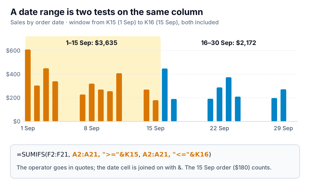
Four habits keep date criteria reliable:
- Keep dates in cells, or build them with DATE.
">="&DATE(2026,9,1)means 1 September everywhere. A typed">=9/1/2026"can be read as 9 January on a computer set to day-first dates. - For a whole month, use "before the first of next month".
">="&DATE(2026,9,1)and"<"&DATE(2026,10,1)catch every September order, $5,807, without worrying whether September has 30 or 31 days. - Watch for times. Exports from point-of-sale and ecommerce systems often store 15 September 2:40 pm, which is later than 15 September and so fails
"<="&K16. Use"<"&K16+1to include the whole last day. - Check that dates are dates. If a date column is left-aligned, it's probably text, and no date criteria will match it.
OR conditions: add SUMIFS together
Since every SUMIFS test must pass, two tests on the same column can never both be true. Asking for prawns and snapper in one SUMIFS returns 0.
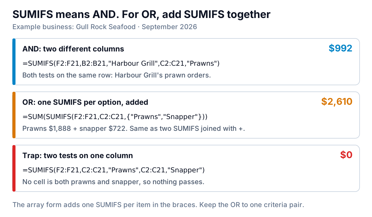
For "prawns or snapper", add two SUMIFS, or let an array constant do it in one formula:
=SUMIFS(F2:F21,C2:C21,"Prawns")+SUMIFS(F2:F21,C2:C21,"Snapper")=SUM(SUMIFS(F2:F21,C2:C21,{"Prawns","Snapper"}))
Both return $2,610: prawns $1,888 plus snapper $722. The braces make SUMIFS run once per item, and SUM adds the results. Keep the OR to one criteria pair; two arrays in one SUMIFS don't combine the way you'd expect. Make sure the options can't overlap, too. "Prawns" or "Shellfish" would count every prawn order twice, because prawns are shellfish.
One formula, a whole summary table
Most of the time you don't want one SUMIFS answer; you want a grid of them, such as sales by customer and category. You can write that grid with a single formula, as long as the dollar signs are in the right places. In the practice workbook the customers run down M2:M6, the categories run across N1:O1, and N2 holds:
=SUMIFS($F$2:$F$21,$B$2:$B$21,$M2,$D$2:$D$21,N$1)Copy it across one column and down four rows and every cell fills in correctly. The data ranges are fully locked, so they never move. $M2 locks the column, so every cell in a row reads that row's customer. N$1 locks the row, so every cell in a column reads that column's category.
| Customer | Shellfish | Fin fish | Total |
|---|---|---|---|
| Harbour Grill | $1,172 | $500 | $1,672 |
| Saltbox Grill | $718 | $514 | $1,232 |
| The Anchor Inn | $454 | $640 | $1,094 |
| Breakwater Café | $417 | $408 | $825 |
| Rockpool Bistro | $0 | $984 | $984 |
| Total | $2,761 | $3,046 | $5,807 |
The grid tells Gull Rock something the raw list hides: Rockpool Bistro buys no shellfish at all, and Harbour Grill's spend leans heavily on prawns. The bottom-right total matches the plain SUM of the Amount column, which proves no order fell through the gaps. If a new customer appears in next month's data and isn't in column M, the grid total drops below the SUM, and that gap is your signal to add a row.
SUMIFS or a pivot table?
Use SUMIFS when you know the questions in advance and want the answers in fixed cells: a summary block at the top of a sheet, a monthly report layout, or one cell that a chart or KPI reads. Each formula is visible and updates the moment the data changes. A pivot table is better when you're exploring: dragging customers against products to see what's there, before you know which numbers matter. Many sheets use both: a pivot table to find the question, then SUMIFS to answer it in the report.
If you work in Google Sheets, the function behaves almost the same; our guide to SUMIFS in Google Sheets covers the differences. For a full worked example of a summary page built on SUMIFS, see our sales report guide.
Common SUMIFS errors and how to fix them
| What you see | Cause | Fix |
|---|---|---|
| #VALUE! | Ranges of different sizes, such as F2:F21 with B2:B20 (row 19 of the Solution sheet) | Make every range cover the same rows; whole columns (F:F, B:B) avoid it |
| #VALUE! after reopening the file | The formula reads another workbook that's closed; Microsoft lists this as a known cause | Open the other workbook and press F9, or copy the data into this one |
| 0 when you expected a total | Cell reference typed inside the quotes (">=K15") | ">="&K15 |
| 0 or too low with text criteria | Trailing spaces or a different spelling ("Harbour Grill " or "Harbor Grill") | Clean the column with TRIM, or match with a wildcard: "Harbo*Grill*" |
| Total too low, no error | Amounts stored as text, which SUMIFS skips | Convert them to numbers |
| Wrong total, no error | Arguments in SUMIF order, so the column you meant to add is being tested instead | Put the sum range first |
| #VALUE! with long criteria | A criteria string over 255 characters | Shorten it, or split it with & |
The sixth row is the classic one if you learned SUMIF first. The two functions put the sum range at opposite ends, and Microsoft's reference calls out the different argument order. Our SUMIF vs SUMIFS guide shows what happens when the order goes wrong, and when SUMIF still makes sense.
When the formulas become a monthly job
For Gull Rock, the real work is the monthly version of this sheet: sales by customer and product, unpaid orders, and a comparison with August. Each month someone pastes in a new export, checks that the ranges still reach the last row, and fixes whichever formula broke.
Parity can do that part from the data itself. Upload the order export as a CSV or Excel file, or connect Shopify, Square or QuickBooks Online directly, and it builds a dashboard with the headline numbers and their trends, charts, what explains them, and a table of what needs attention, such as unpaid orders. Every number is checked against queries on the full dataset before you see it, and you can export the result to Excel. When next month's file arrives, you update the dashboard with it instead of rebuilding the formulas.
Upload your order export and get a checked dashboard of sales by customer and product. Build a report from your data free
Before you rely on any SUMIFS you write, run the same check the practice workbook uses: split a total into parts that can't overlap, such as paid plus unpaid or the first half of the month plus the second, and make sure the parts add back to the plain SUM. If they do, your criteria are catching every row they should.