SUMIFS in Google Sheets adds up the numbers in one column for the rows that meet every condition you give it: =SUMIFS(F2:F25, D2:D25, "Wedding", G2:G25, "Unpaid") totals the amounts in column F where column D says Wedding and column G says Unpaid. The range to add always comes first, followed by pairs of a range to check and the condition to check it against.
That's the syntax Google gives on its SUMIFS help page: SUMIFS(sum_range, criteria_range1, criterion1, [criteria_range2, criterion2, …]). Getting the conditions right is the hard part: dates, "not equal to", partial text, and "this or that" each need a slightly different way of writing. This guide works through each one on a real-looking order book, then builds the one summary table most small businesses want, and ends with the reasons SUMIFS returns 0 when it shouldn't.
The example business is Wildflower Wedding Florals, a fictional florist. Its order book holds 24 invoice lines for events from May to September 2026: event date, invoice number, client, event type (Wedding, Elopement or Corporate), item, amount and status (Paid, Deposit paid or Unpaid). Every line adds up to $17,655. Download the practice workbook (.xlsx); upload it to Google Drive and open it in Sheets, or use File > Import. It also opens in Excel. The Practice sheet has nine questions with the expected answers beside them, and the Solution sheet has the formulas.
How SUMIFS in Google Sheets reads a formula
Read a SUMIFS formula from left to right as a sentence: "add up these amounts, where this column is this, and that column is that." Every pair narrows the rows further. Google's help puts it plainly: to be counted, a row has to meet all the criteria.
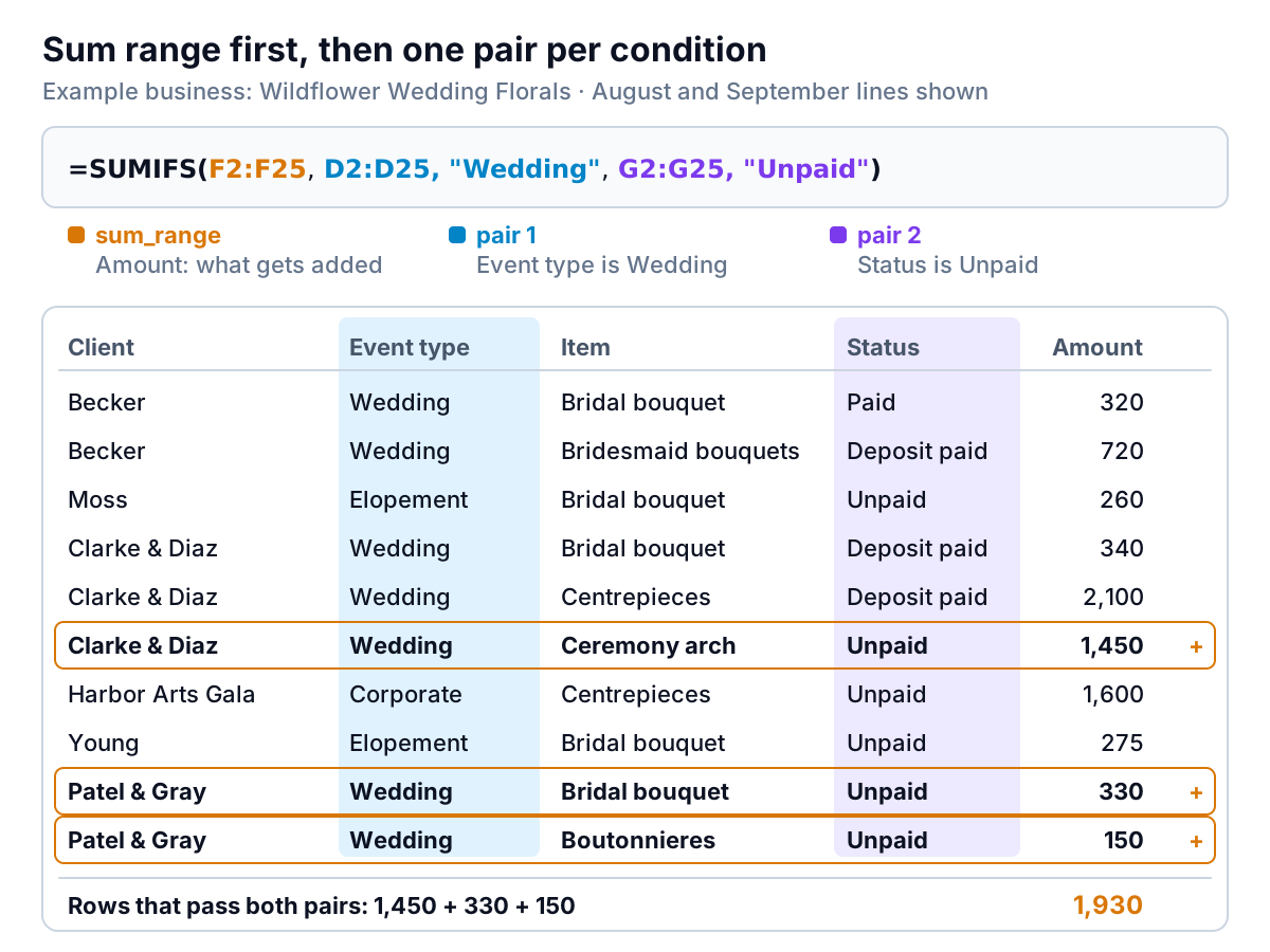
On the florist's book, =SUMIFS(Orders!F2:F25, Orders!D2:D25, "Wedding") returns $13,060, all the wedding work booked. Adding the second pair, Orders!G2:G25, "Unpaid", narrows it to three lines: the Clarke & Diaz ceremony arch ($1,450) and the Patel & Gray bouquet and boutonnieres ($330 and $150). That's $1,930 of wedding money still to collect.
Three rules hold for every SUMIFS:
- All the ranges must be the same size. F2:F25 with D2:D25 is fine; F2:F25 with D2:D30 is an error.
- Text conditions go in quotation marks. "Wedding", not Wedding. Without quotes, Sheets looks for a named range called Wedding.
- Matching isn't case-sensitive. "wedding" finds Wedding.
The criteria cheat sheet
Nearly every SUMIFS question comes down to how you write the condition. Google documents the operators and wildcards on its SUMIF page, which SUMIFS shares. Here they are with the florist's numbers.
| You want | Condition | Formula (sum range F, Orders sheet) | Result |
|---|---|---|---|
| Exactly a word | "Wedding" | =SUMIFS(F2:F25, D2:D25, "Wedding") | $13,060 |
| Anything except a word | "<>Corporate" | =SUMIFS(F2:F25, G2:G25, "Unpaid", D2:D25, "<>Corporate") | $2,465 |
| Contains some text | "*bouquet*" | =SUMIFS(F2:F25, E2:E25, "*bouquet*") | $4,135 |
| A number threshold | ">=1000" | =SUMIFS(F2:F25, F2:F25, ">=1000") | $12,040 |
| A value typed in another cell | B13 | =SUMIFS(F2:F25, D2:D25, B13) | Whatever B13 says |
| Not equal to a cell | "<>"&B14 | =SUMIFS(F2:F25, D2:D25, B13, G2:G25, "<>"&B14) | $7,140 (Wedding, not Paid) |
The formulas in the table leave out the Orders! prefix to fit; the workbook has the full versions.
Two of these deserve a closer look. The "contains" condition uses the asterisk wildcard, which stands for any run of characters, so "*bouquet*" catches Bridal bouquet and Bridesmaid bouquets. A question mark stands for exactly one character. To match a real asterisk or question mark, put a tilde in front of it (~*).
The cell-reference condition is the one to build habits around. When an operator and a cell are combined, the operator goes in quotes and the ampersand joins it to the cell: "<>"&B14, ">="&H1. Writing "<>B14" instead compares against the literal text B14 and quietly returns the wrong total.
SUMIFS with dates in Google Sheets
Most real SUMIFS questions are about a period: this month, last quarter, since the season started. A date condition is just a number condition, because Sheets stores dates as numbers, so the same operator-and-ampersand rule applies.
For everything in June 2026, use a start date and the first day of the next month:
=SUMIFS(Orders!F2:F25, Orders!A2:A25, ">="&DATE(2026,6,1), Orders!A2:A25, "<"&DATE(2026,7,1))That returns $5,515: eight lines across four June events. Notice that the same column, A, appears twice, once for each end of the range. That's allowed, and it's how you write "between".
The alternative end condition is "<="&EOMONTH(DATE(2026,6,1),0), which gives the last day of the month. EOMONTH returns midnight on that day, so if your dates carry times (some booking and payment exports do), a sale at 3pm on 30 June is left out. "Less than the first of next month" never has that problem.
For rolling periods, swap the fixed dates for TODAY(): ">="&TODAY()-30 for the last 30 days, or ">="&EOMONTH(TODAY(),-1)+1 for the current month to date.
">=6/1/2026" sometimes works and sometimes doesn't, depending on the spreadsheet's locale (File > Settings). In a UK-locale sheet, 6/1/2026 is 6 January. DATE(2026,6,1) means 1 June everywhere.OR conditions: this event type or that one
SUMIFS only does AND. Every pair must be true. "Weddings or elopements in September" needs a workaround, and there are three good ones.
Add two SUMIFS together. The simplest, and the easiest to read six months later:
=SUMIFS(F2:F25, D2:D25, "Wedding", A2:A25, ">="&DATE(2026,9,1), A2:A25, "<"&DATE(2026,10,1))+SUMIFS(F2:F25, D2:D25, "Elopement", A2:A25, ">="&DATE(2026,9,1), A2:A25, "<"&DATE(2026,10,1))
Give SUMIFS a list and add up the answers. Put both event types in curly brackets and SUMIFS returns one total for each. In Google Sheets you wrap it so the list is evaluated as an array, with ARRAYFORMULA or SUMPRODUCT:
=SUMPRODUCT(SUMIFS(F2:F25, D2:D25, {"Wedding","Elopement"}, A2:A25, ">="&DATE(2026,9,1), A2:A25, "<="&EOMONTH(DATE(2026,9,1),0)))Both return $4,645: $4,370 of weddings and $275 of elopements. The workbook uses the SUMPRODUCT version because it works in Excel too. Only put one list in a formula; two lists in different conditions pair up item by item instead of covering every combination.
Use FILTER with REGEXMATCH. This one is Sheets-only, and it's the most flexible when the list gets long:
=SUM(FILTER(F2:F25, REGEXMATCH(D2:D25, "Wedding|Elopement")))The vertical bar means "or", per Google's REGEXMATCH page. Across the whole season this gives $14,055. One catch: REGEXMATCH is case-sensitive, unlike SUMIFS, and "Wedding" also matches "Wedding party". Add ^ and $ around the pattern ("^(Wedding|Elopement)$") to match whole cells only.
One formula, a whole monthly summary
The real payoff from SUMIFS in Google Sheets is a summary table that fills itself: months down the side, event types across the top, one formula copied into every cell. The trick is the dollar signs.
=SUMIFS(Orders!$F$2:$F$25, Orders!$D$2:$D$25, B$17, Orders!$A$2:$A$25, ">="&$A18, Orders!$A$2:$A$25, "<="&EOMONTH($A18,0))Type it once in B18 and copy it across and down. The data ranges are fully locked ($F$2:$F$25). B$17 locks the row, so every cell reads its event type from the header row, while the column moves as you copy right. $A18 locks the column, so every cell reads its month from column A, while the row moves as you copy down. Column A holds the first day of each month, formatted to show "May 2026".
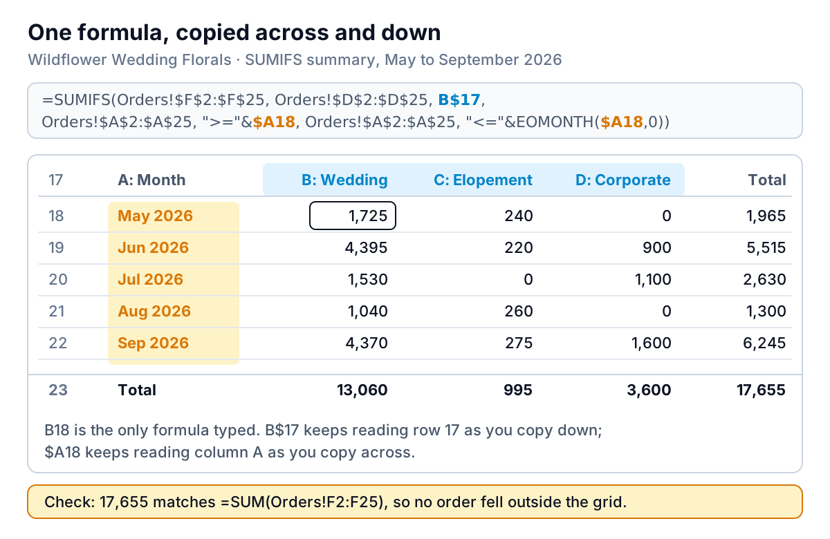
The grid tells the florist things the order book doesn't. June and September carry the season, at $5,515 and $6,245. Corporate work is small but lumpy: $3,600 from three events, and $2,700 of it still unpaid. Elopements total just $995 across four bookings. Always add a grand total to a grid like this and check it against a plain SUM of the amount column. If they differ, some rows fell outside every bucket, usually because of a date stored as text or a misspelled event type.
If you'd rather drag and drop than write a formula, the same table is a pivot table with Event type in Columns and the date grouped by Year-Month in Rows; our guide to the pivot table in Google Sheets walks through it. Formulas win when you want the layout fixed and the cells referenced elsewhere, as on a Google Sheets dashboard.
Why SUMIFS returns 0 (or an error), and the fix
| Symptom | Cause | Fix |
|---|---|---|
| 0 when there are clearly matching rows | Amounts stored as text (left-aligned, often from a CSV); SUMIFS skips text | Format > Number > Number, or use a helper column with =VALUE(F2) |
| 0 for a date range | Dates stored as text, so they're not "greater than" anything | Convert with DATEVALUE, or re-import with the right locale |
| 0 for a text match | Trailing spaces ("Wedding ") or a different spelling | Data > Data cleanup > Trim whitespace, or match with "Wedding*" |
| A wrong total with a cell condition | Operator and cell inside the same quotes: ">=H1" | ">="&H1 |
| An error about array arguments of different size | Ranges of different lengths, e.g. F2:F25 and D2:D24 | Make every range cover the same rows |
| A total of the wrong column | Argument order from SUMIF, where the sum range comes last | In SUMIFS the sum range is always first |
| Totals change when copied | Ranges not locked with $ | $F$2:$F$25 for data, one $ for headers |
| An OR total that looks too small | The {"Wedding","Elopement"} list wasn't evaluated as an array | Wrap in SUMPRODUCT or ARRAYFORMULA |
Two habits prevent most of these. Use open-ended ranges such as Orders!F2:F in Sheets so new rows are included automatically, as long as every range in the formula is open-ended in the same way. And keep a "check" cell that compares your grid's grand total with =SUM(Orders!F2:F).
When the order book outgrows the formulas
SUMIFS is the right tool for a monthly summary you control cell by cell. It gets heavier when the questions multiply: by planner, by venue, by item, unpaid over 30 days, this season against last. Each new question is another grid, and each grid is another set of ranges to keep in step when the data grows.
That's the point where Parity can help. Connect Google Sheets directly, or upload your order export as a CSV or Excel file, and it builds a dashboard: headline numbers with their trends, charts, what explains them, and a table of what needs attention, such as unpaid balances by event. Every number is checked against queries on the full dataset before you see it, so the totals tie back to your book. You refine it by chat ("revenue by event type and month", "show only unpaid"), and update it with a newer file. For the wider picture, our sales report guide covers which numbers belong on the monthly page.
Connect your order sheet and get a checked dashboard of bookings, revenue and unpaid balances. Build a report from your data free
Either way, the habit that matters is the same one the grid teaches: make every total prove itself against the raw data before you act on it.