XLOOKUP in Google Sheets finds a value in one column and returns the matching value from another: =XLOOKUP(A4, Catalogue!A2:A11, Catalogue!B2:B11, "Not in catalogue") looks up the SKU in A4 among the catalogue's SKUs and returns its product name, or "Not in catalogue" if there's no match. The full syntax is XLOOKUP(search_key, lookup_range, result_range, missing_value, match_mode, search_mode), and only the first three arguments are required.
Google added XLOOKUP to Sheets in August 2022, along with XMATCH and LAMBDA. It works almost exactly like Excel's version, and the few differences are the ones that trip people up when a file moves between the two. This guide covers every argument on one practical job, a quote for a contractor, then the Sheets-specific behaviour and the errors you'll actually see.
The example business is Lumen Lighting Co., a fictional lighting supplier with a 10-product catalogue, a quantity discount table and a log of price changes. Download the practice workbook (.xlsx), then upload it to Google Drive and open it in Sheets (or use File > Import in a blank sheet). The Practice sheet has yellow cells to fill in with the expected answers beside them; the Solution sheet has the working formulas.
The six arguments of XLOOKUP in Google Sheets
Here's each argument, with Google's definition from the XLOOKUP help page and what it means on Lumen's quote.
| Argument | What it is | On Lumen's quote |
|---|---|---|
search_key | The value to find | The SKU typed on the quote, e.g. A4 = LL-1004 |
lookup_range | Where to look; must be a single row or a single column | Catalogue!A2:A11, the SKU column |
result_range | What to return; the same number of rows (or columns) as lookup_range | Catalogue!B2:B11 for the name, F2:F11 for the price |
missing_value | Optional. What to show if there's no match (#N/A by default) | "Not in catalogue" |
match_mode | Optional. 0 exact (default), 1 exact or next greater, -1 exact or next lesser, 2 wildcard | -1 for the discount tiers |
search_mode | Optional. 1 first to last (default), -1 last to first, 2 binary search ascending, -2 binary search descending | -1 to find the latest price change |
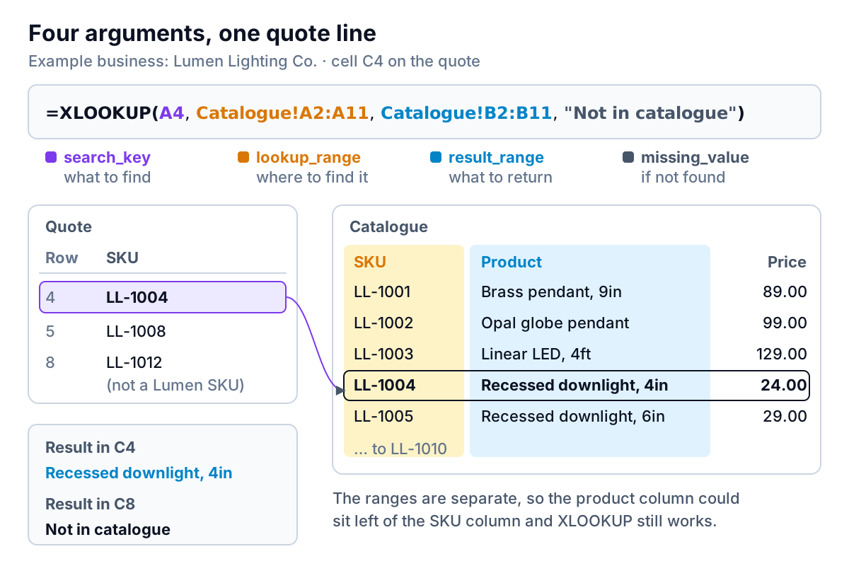
Build the quote: exact matches and a missing value
A contractor has asked for five items. The quote sheet holds the SKU in column A and the quantity in column B. Three XLOOKUPs fill the rest of each row:
C4: =XLOOKUP(A4, Catalogue!$A$2:$A$11, Catalogue!$B$2:$B$11, "Not in catalogue")D4: =XLOOKUP(A4, Catalogue!$A$2:$A$11, Catalogue!$F$2:$F$11, 0)E4: =XLOOKUP(B4, Tiers!$A$2:$A$5, Tiers!$B$2:$B$5, 0, -1)
The dollar signs keep the ranges fixed when you copy the formulas down to row 8. The line total in F4 is =B4*D4*(1-E4).
The missing_value argument does the job IFERROR used to. For the price, Lumen uses 0 rather than text, so the line total still calculates (to $0.00) and the quote total doesn't break. On the product name, "Not in catalogue" tells whoever reads the quote exactly what went wrong. The contractor's fifth line, LL-1012, isn't a Lumen SKU, and that's what the quote shows.
The results: 40 of LL-1004 recessed downlights at $24.00 less 8% = $883.20; 12 of LL-1008 track heads at $45.00 less 5% = $513.00; 3 of LL-1001 brass pendants at $89.00 = $267.00; 8 of LL-1009 dimmer switches at $27.00 = $216.00; and LL-1012 at $0.00. Quote total: $1,879.20.
Approximate match for price breaks and tiers
Lumen gives quantity discounts: 1 to 9 units no discount, 10 to 24 units 5%, 25 to 49 units 8%, 50 or more 12%. The Tiers sheet stores only the starting quantity of each band (1, 10, 25, 50) and its discount. That's the standard layout for any tiered table: shipping bands, commission rates, tax brackets.
With match_mode set to -1, XLOOKUP looks for the quantity exactly and, if it isn't there, takes the next lesser value. A quantity of 40 isn't in the table, so XLOOKUP falls back to 25 and returns 8%. Twelve falls back to 10 and returns 5%. Three falls back to 1 and returns 0%.
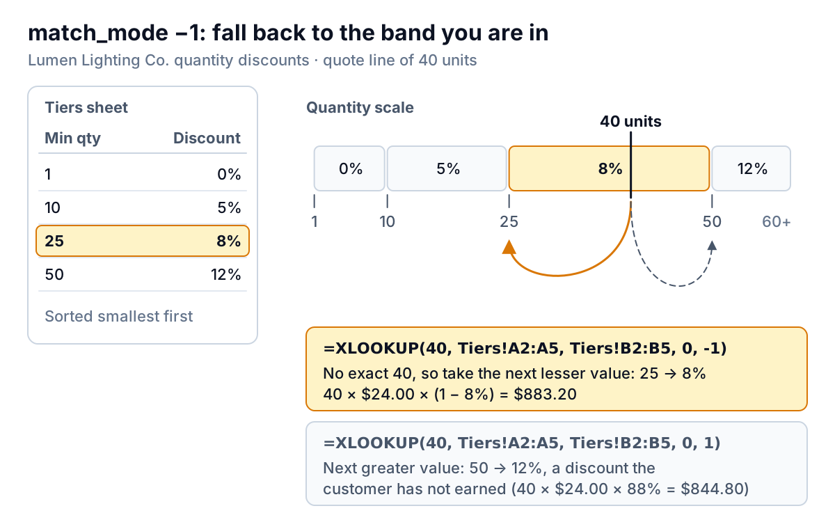
Two things to get right. First, choose -1 for a table of starting points ("from 25 units"). If your table lists upper limits instead ("up to 24 units"), use 1. Second, XLOOKUP's approximate match doesn't need the table sorted when search_mode is left at its default, unlike VLOOKUP with TRUE. Sorting still makes the table easier for a person to check, so keep it sorted anyway.
Search last to first, wildcards, left lookups and several columns
The latest entry: search_mode -1
The Price history sheet logs every list-price change, oldest first. LL-1004 appears three times: $22.00 from 5 January, $23.00 from 1 June and $24.00 from 15 September 2026. A plain XLOOKUP returns the first match it finds, which is the January price of $22.00. Setting search_mode to -1 searches from the bottom up and returns the most recent one:
=XLOOKUP("LL-1004", 'Price history'!B2:B8, 'Price history'!C2:C8, , 0, -1)That returns $24.00. The empty argument between the commas skips missing_value. The same trick finds a customer's last order, a job's latest status or the most recent stock count, as long as the log is in date order.
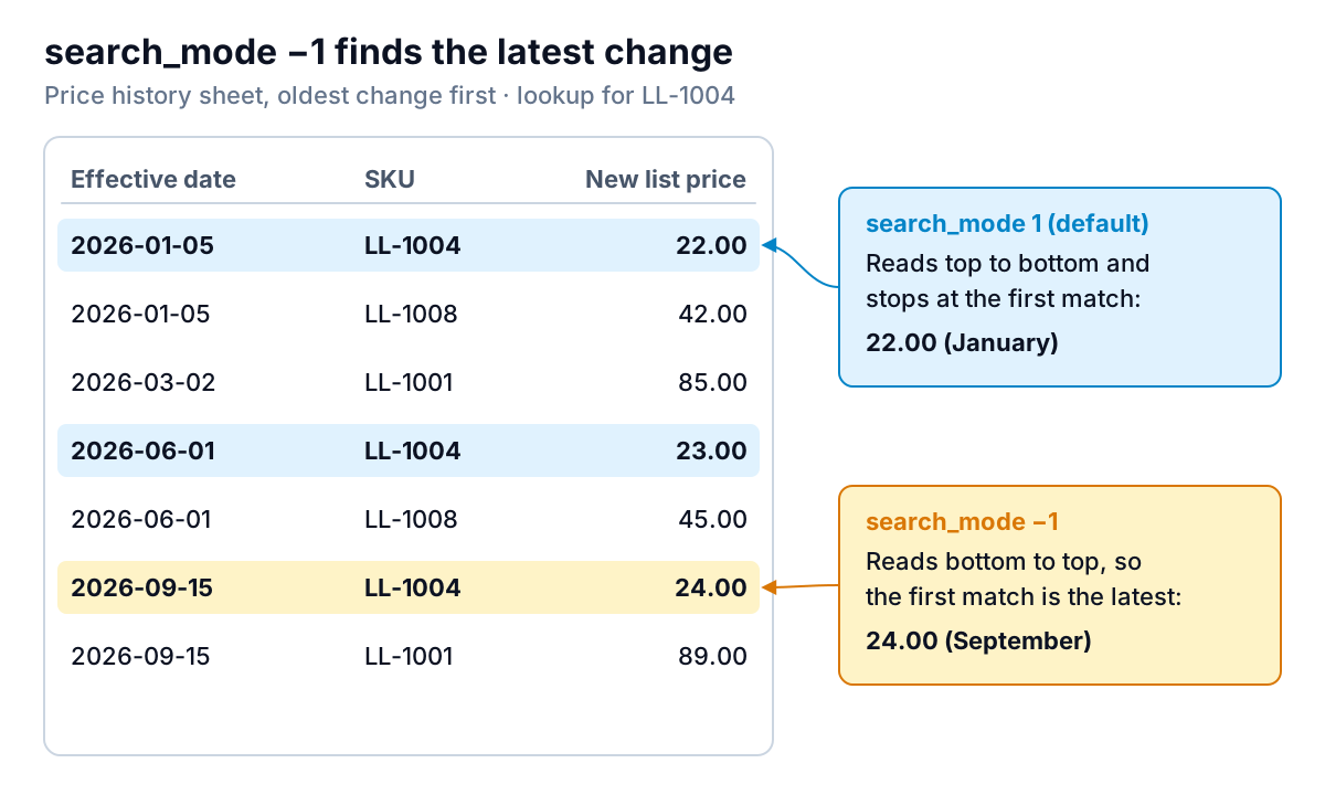
Leave search modes 2 and -2 (binary search) alone unless your lookup range is large and sorted. On unsorted data a binary search doesn't fail with an error; it returns a wrong answer that looks right.
Wildcards: match_mode 2
With match_mode 2, an asterisk stands for any run of characters and a question mark for one character. =XLOOKUP("*globe*", Catalogue!B2:B11, Catalogue!A2:A11, "None", 2) returns LL-1002, the opal globe pendant. To search for a real asterisk or question mark, put a tilde in front of it (~*). Without match_mode 2, the asterisk is treated as an ordinary character and the lookup returns #N/A.
Lookups to the left
Because the ranges are separate, the result can sit left of the lookup column. =XLOOKUP("Smart dimmer", Catalogue!B2:B11, Catalogue!A2:A11) returns LL-1010. With VLOOKUP you'd have to rearrange the columns; our VLOOKUP in Google Sheets guide shows the workarounds if you're stuck with an older file.
Several columns at once, and two-way lookups
Google's help notes that if result_range is more than one column, XLOOKUP returns the whole row at the match. =XLOOKUP(B21, Catalogue!A2:A11, Catalogue!B2:D11) with LL-1007 in B21 fills three cells across: Bollard light, 24in; Outdoor; Harbour Lamps. Leave those cells empty, or the formula can't spill into them.
Nest one XLOOKUP inside another for a two-way lookup. The inner one finds the column by its header; the outer one finds the row:
=XLOOKUP("LL-1007", Catalogue!A2:A11, XLOOKUP("In stock", Catalogue!A1:G1, Catalogue!A2:G11))That returns 9. Change "In stock" to "List price" and the same formula returns 149.
How XLOOKUP in Google Sheets differs from Excel
If your bookkeeper works in Excel and you work in Sheets, these are the differences worth knowing:
| Topic | Google Sheets | Excel |
|---|---|---|
| Who has it | Every Sheets user since August 2022 | Excel for Microsoft 365, Excel 2021 and Excel 2024, per Microsoft Support; not Excel 2019 or earlier |
| Argument names | search_key, lookup_range, result_range, missing_value | lookup_value, lookup_array, return_array, if_not_found. Same order, same behaviour |
| A result that can't spill | #REF! with "Array result was not expanded because it would overwrite data" | #SPILL! |
| A whole column of search keys | Wrap it: =ARRAYFORMULA(XLOOKUP(A4:A8, …)). Ctrl+Shift+Enter adds ARRAYFORMULA for you | Spills on its own in Microsoft 365 |
| Open-ended ranges | A2:A works, so new rows are included | Use a full column or an Excel table |
| Connected Sheets (BigQuery) | search_mode isn't supported | Not applicable |
The practical rule for XLOOKUP in Google Sheets files that leave Sheets: if anyone opening your file uses Excel 2019 or older, every XLOOKUP becomes #NAME? when they download it. For files that travel, either keep VLOOKUP or INDEX/MATCH (our XLOOKUP vs VLOOKUP comparison covers when that's worth it) or paste the results as values before sending.
XLOOKUP errors in Google Sheets and how to fix them
| What you see | Likely cause | Fix |
|---|---|---|
| #N/A on a SKU you can see in the list | One side is a number, the other is text (1004 vs "1004"), often from a CSV export | Match the types: =XLOOKUP(TO_TEXT(A4), …) or =XLOOKUP(VALUE(A4), …) |
| #N/A that looks impossible | A trailing space ("LL-1004 ") | Data > Data cleanup > Trim whitespace, or look up TRIM(A4) |
| An error instead of any result | lookup_range and result_range are different sizes, e.g. A2:A11 and B2:B12 | Make both ranges start and end on the same rows |
| #REF! "would overwrite data" | A multi-column result has something in its way | Clear the cells to the right of the formula |
| The wrong tier or band | match_mode 1 where -1 was needed (or the reverse) | -1 for "from" thresholds, 1 for "up to" thresholds |
| An old value instead of the latest | Default search_mode returns the first match | search_mode -1 on a log kept oldest-first |
| A plausible but wrong answer | Binary search (2 or -2) on unsorted data | Go back to search_mode 1 or -1, or sort the range |
| #NAME? after downloading to Excel | The Excel version predates XLOOKUP | Paste values, or use INDEX/MATCH in shared files |
XLOOKUP isn't case-sensitive: "ll-1004" finds LL-1004. If case matters, you need a different approach, such as FILTER with EXACT.
When lookups are holding a report together
XLOOKUP is the right tool for joining two lists: a quote and a catalogue, an order export and a product list, an invoice list and a customer table. Where it starts to strain is when the lookups are there to stitch together a monthly report from three exports, and each month someone pastes new data in and hopes the ranges still reach.
If that's your situation, Parity can take the exports directly. Connect Google Sheets, Shopify, QuickBooks Online or Square, or upload the CSV or Excel files, and it builds a dashboard with headline numbers and their trends, charts, what explains them, and a table of what needs attention. Every number is checked against queries on the full dataset before you see it. You refine it by chat ("show revenue by product category", "flag items out of stock"), and update it with next month's file instead of re-checking every lookup. For the bigger picture of what to put on that page, see our guide to inventory dashboards.
Upload your order and product exports and get a checked dashboard that joins them for you. Build a report from your data free
For everything smaller, the quote sheet in the workbook is a good template to keep: one SKU column, one quantity column, and three XLOOKUPs that tell you plainly when a part number doesn't exist.