How to Refresh a Pivot Table (and Why New Rows Don't Show Up)

To refresh a pivot table in Excel, right-click anywhere inside it and choose Refresh, or click in it and press Alt+F5. To refresh every pivot table in the workbook at once, use Refresh All (Ctrl+Alt+F5, or the Refresh All button on the Data tab).

That takes five seconds. The reason people search for how to refresh a pivot table is usually different: they refreshed, and the numbers still look wrong. The new rows aren't there, a column vanished, or the formatting reset. This guide covers the refresh options first, then each of those problems with its fix, using a small pottery studio's sales as the example.

Download the practice workbook (.xlsx). It has 25 September sales on a Practice sheet, 6 October sales to paste in, and a Solution sheet with the expected totals before and after, worked out with SUMIFS. You build the pivot yourself (file generators can't create real PivotTables), which is how you'll see the problems below happen.

Why a pivot table needs refreshing at all

A pivot table doesn't read your cells every time you look at it. When you build one, Excel copies the source data into a hidden store called the pivot cache, and the pivot summarises the cache. Change a number in the source and the cache still holds the old one until you refresh.

This is different from formulas. A SUMIFS updates the moment you change a cell. A pivot waits. Google Sheets behaves like formulas here: Google's help says its pivot table refreshes any time you change the source data it's drawn from. Excel is catching up: Microsoft is rolling out an Auto Refresh setting, covered below, but in most copies of Excel today you still refresh by hand.

Here's the example. Cinder Ceramics Studio, an example business, sells wheel classes, open-studio memberships, kiln firings for members' pieces, and finished pottery. The owner keeps a sales list and a pivot of Sum of Amount by Type. On 3 October she pastes in the first six October sales and refreshes. The Grand Total doesn't move from $2,360. Why is the first problem below.

How to refresh a pivot table: the five options

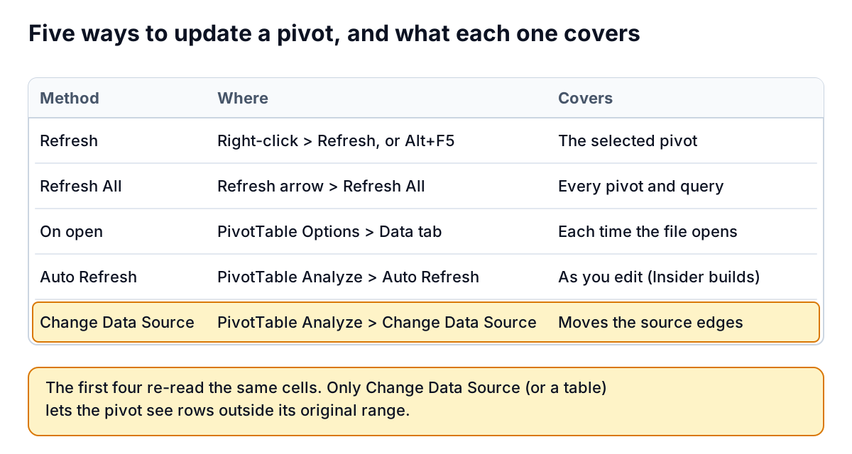
These come from Microsoft's page on refreshing PivotTable data, with menu names from Excel for Microsoft 365 on Windows.

1. Refresh one pivot. Click inside it, then PivotTable Analyze > Refresh, or right-click > Refresh, or Alt+F5. On a Mac, Control-click > Refresh.
2. Refresh All. Click the arrow under the Refresh button and choose Refresh All, or use Data > Refresh All. Microsoft's shortcut list gives Ctrl+Alt+F5 to refresh all data in the workbook. This also refreshes Power Query queries and other connections, which can take a while on a big file.
3. Refresh when the file opens. Click in the pivot, choose PivotTable Analyze > Options, go to the Data tab and tick Refresh data when opening the file. Good for a workbook you open once a week to read.
4. Auto Refresh. Microsoft's page describes a PivotTable Auto Refresh setting that updates the pivot as soon as its in-workbook source changes, and lists it as available to Microsoft 365 Insider participants at the time of writing. If you have it, there's an Auto Refresh button on the PivotTable Analyze tab. It's set per data source, so all pivots built from the same data turn on or off together. It doesn't apply to external sources such as databases.
5. Change Data Source. Not a refresh, but the fix when a refresh can't see your new rows. Next section.

Which option to use

A simple rule for deciding how to refresh a pivot table in a business file:

• One pivot, one quick check: Alt+F5.
• A report with several pivots or charts: always Refresh All before you read or send it. Refreshing one pivot and not the next is how a summary page ends up showing two different totals for the same month.
• A file other people open to read: turn on refresh when opening, so nobody reads last week's numbers because they didn't know to refresh.
• A file you edit all day: Auto Refresh if your Excel has it. If not, get in the habit of refreshing before you look at the pivot, not after.

New rows don't show up after refresh

This is the most common refresh problem by a distance, and it's what happened at the studio. She built her pivot by selecting A1:D26 and choosing Insert > PivotTable. Excel stored that exact address as the source. When she pasted six October rows into rows 27 to 32 and refreshed, Excel dutifully re-read A1:D26. The new rows were outside it.

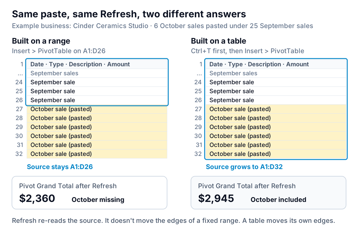
There are two fixes. Do the second one once and you won't need the first again.

Quick fix: widen the range. Click in the pivot, choose PivotTable Analyze > Change Data Source > Change Data Source, change the range to include the new rows (A1:D32), and select OK. Microsoft's guide to changing the source notes one limit: if the pivot is based on the workbook Data Model, you can't change its source this way. You'll be back here next month.

Lasting fix: make the source an Excel table.

1. Click any cell in the sales data and press Ctrl+T. Tick My table has headers and select OK. Excel names the table (Table1, unless you rename it on the Table Design tab; something like Sales is easier to recognise).
2. Click in the pivot, choose PivotTable Analyze > Change Data Source > Change Data Source, and type the table name in the Table/Range box instead of an address.
3. Select OK, then refresh.

From now on, anything you paste or type directly under the last row becomes part of the table, because an Excel table extends itself when you add data next to it. The pivot reads "the Sales table", wherever its edges are today. At the studio, the Grand Total goes from $2,360 to $2,945 on the next refresh.

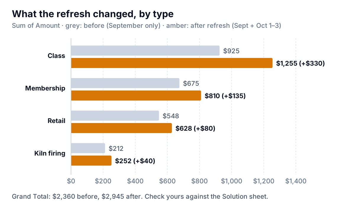
Two habits keep this working. Paste new rows directly under the table, with no blank row in between. And if you replace the data every month with a fresh export, paste the new rows into the existing table (select the table's first data cell and paste) rather than pasting the export onto a new sheet.

Six other things that go wrong when you refresh

1. "A PivotTable report cannot overlap another PivotTable report." The refreshed pivot is bigger than before (a new month, a new product) and would run into a second pivot on the same sheet. Move one of them, or give each pivot its own sheet. The same applies to any data sitting right below or beside a pivot: Excel asks before overwriting it.

2. A field disappears. You renamed a column header in the source, say "Amount" to "Amount ($)". To the pivot that's a field that no longer exists, so it drops out of the layout on refresh. Rename it back, or drag the new field into place again. Any calculated field whose formula uses the old name needs editing too. Keep headers stable in any export you refresh into.

3. Column widths and formatting reset. Open PivotTable Analyze > Options, and on the Layout & Format tab untick Autofit column widths on update and tick Preserve cell formatting on update. Microsoft documents both in its PivotTable options reference. Apply number formats through the value field (right-click > Number Format) rather than by formatting cells, and they survive refreshes.

4. Old items hang around in the filter list. The studio renamed "Kiln firing" to "Firing", and the old name still shows in the filter drop-down with nothing under it. The pivot cache keeps deleted items by default. In PivotTable Options, on the Data tab, set Number of items to retain per field to None, select OK, then refresh.

5. The total is too low, with no error. A pasted row has its amount stored as text, such as "$40" typed with the symbol, or a number from a web export. Sum skips text silently. Look for cells aligned to the left in the Amount column, convert them to numbers, and refresh. Our guide to cleaning data in Excel covers this and other export problems.

6. "Data source reference is not valid." The pivot points at a sheet, range or table that's been renamed, moved or deleted. Use Change Data Source to point it at the right place. If the data now lives in another workbook, open that workbook first.

A refresh routine for a monthly report

If a pivot feeds a report you send each month, knowing how to refresh a pivot table is only half of it. A two-minute routine stops most surprises:

1. Paste the new rows under the table. No blank row. Check the table's border now includes them.
2. Refresh All, so every pivot and chart in the file uses the same data.
3. Check one total by hand. Pick a number you can verify elsewhere, such as the month's sales in your till or accounting system, and compare. A row count works too: the pivot's Count of Date should equal the number of rows in the table.
4. Scan for (blank). A "(blank)" row label means some rows are missing a value in that field. Find them in the source before you send anything.
5. Re-apply the sort. If new items appeared, check they landed where you expect. Our guide to sorting a pivot table explains which sorts survive a refresh and which don't.

If you're new to pivots, start with what a pivot table is and how to create one; it uses the same Rows, Columns and Values terms as this guide.

The routine is fine for one file. It wears thin when the monthly job is "export from the booking system, export from the till, paste both, refresh, fix whatever broke". That's the job Parity is built for. Upload the exports (or connect a tool like Square, Shopify or Google Sheets directly) and Parity builds a dashboard with the headline numbers, their trends and what explains them, checking every number against the full dataset first. Next month you update it with the newer file instead of re-pasting, and you can still export to Excel. For a spreadsheet-only version, our Excel dashboard templates are built on tables for the same reason this post recommends them.

Whatever you use, the test after any refresh is the same: does one number you trust match? If it does, the rest probably does too. If it doesn't, start with the source range.