To add a pivot table calculated field in Excel, click inside the pivot, go to PivotTable Analyze > Fields, Items & Sets > Calculated Field, type a name, enter a formula such as =(Revenue-Cost)/Revenue, and click Add, then OK. The new field appears in Values, and it calculates from the sums of the fields you name, row by row of the pivot, never line by line of your data.
That last sentence is the one to remember. It's why a calculated field gets margin percentages right where averaging a margin column gets them wrong, and it's also why some perfectly reasonable formulas return nonsense. This guide shows both with a beekeeping supplier's spring orders, then covers editing, deleting, and when a calculated item or a measure is the better tool.
Download the practice workbook (.xlsx). The Practice sheet holds 23 order lines in a table called Lines. You build the pivot and the calculated fields yourself (file generators can't create real PivotTables), then check each result on the Solution sheet, where the expected numbers, and the wrong ones, are worked out with SUMIFS and SUMPRODUCT.
How to add a pivot table calculated field
Honeycomb Bee Supply, an example business, sells hive kits, bee suits, smokers, frames and honey jars through three channels: its online shop, a weekend market stall, and wholesale to garden centres. Each order line in its export has Qty, Unit price and Unit cost, and the practice table adds Revenue (Qty × Unit price) and Cost (Qty × Unit cost) as columns.
The owner wants gross profit and margin by channel. The pivot has Channel in Rows and Revenue and Cost in Values. Neither Gross profit nor Margin % exists in the data, so she adds them. The steps follow Microsoft's guide to calculating values in a PivotTable, which calls the tab "Analyze" (its name in Excel 2016 and earlier); in Microsoft 365 it's PivotTable Analyze.
- Click any cell in the pivot.
- Choose PivotTable Analyze > Fields, Items & Sets > Calculated Field.
- In Name, type
Gross profit. - In Formula, delete the 0 after the equals sign. Double-click Revenue in the Fields list (or select it and click Insert Field), type a minus sign, then double-click Cost. The box reads
= Revenue - Cost. - Click Add. Repeat with the name
Margin %and the formula=(Revenue - Cost) / Revenue, click Add again, then OK. - Right-click a Margin % value, choose Number Format, and pick Percentage with one decimal place.
Field names that contain spaces, numbers or symbols need single quotes: ='Unit price' * 1.1. Microsoft's rules also say you can use constants and operators, but not cell references, defined names or array functions, and you can't refer to totals such as Grand Total. That rules out "multiply by the rate in cell B1"; type the rate into the formula instead.
Check yours against Solution table A: Market stall 49.3%, Online 44.2%, Wholesale 28.0%, and 36.8% for the Grand Total.
Why a calculated field sums first, and why that's right for margin
Microsoft states the rule plainly: "Formulas for calculated fields operate on the sum of the underlying data for any fields in the formula." For the Online row, Excel first adds up Revenue for the nine online lines ($9,217) and Cost for the same lines ($5,147), and only then applies the formula: ($9,217 − $5,147) ÷ $9,217 = 44.2%. At the Grand Total it does the same with all 23 lines: $8,589 of gross profit on $23,370 of revenue, 36.8%.
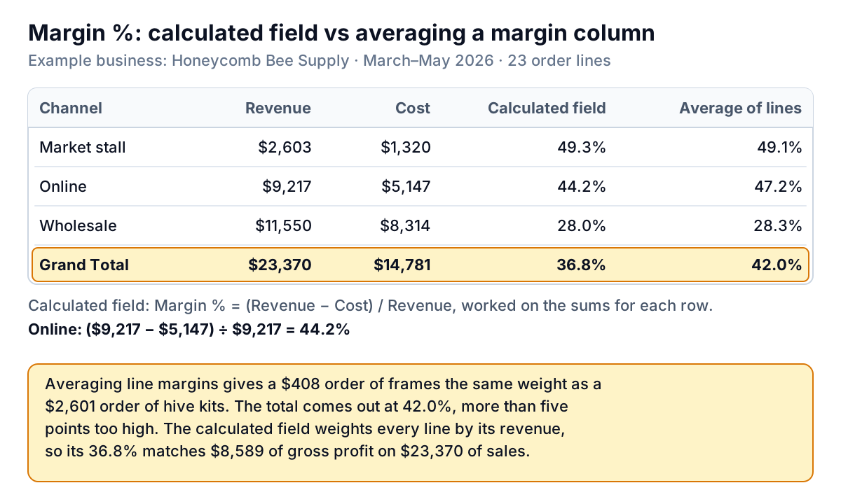
That is the correct margin. Compare the method many people try first: add a Line margin column to the data, put it in Values and switch it from Sum to Average. Every line then counts equally. A $408 order of frames gets the same say as a $2,601 order of hive kits, and the overall figure comes out at 42.0%, more than five points too high. (Summing that column is worse: the nine online lines add up to well over 400%.)
The gap is biggest where line sizes vary most. Wholesale, with uniformly large orders, barely moves (28.0% against 28.3%). Online, where small accessory orders sit next to big hive-kit orders, moves three points. If you're comparing channels to decide where to put effort, three points is enough to make the wrong call. Our guide to calculating gross margin covers the formula itself and what a healthy number looks like.
Once Margin % is in the pivot, you can rank channels by it: right-click a margin value and choose Sort > Sort Largest to Smallest. Our guide to how to sort a pivot table explains which sorts survive a refresh.
When "sums first" gives the wrong answer
The same rule that makes margin right makes two other common formulas wrong.
Multiplying two columns
Suppose the data had no Revenue column, so the owner creates a calculated field =Qty * 'Unit price'. Excel sums Qty for the online lines (78 units), sums Unit price for the same lines ($1,243, a number that means nothing), and multiplies them: $96,954. Real online revenue is $9,217.
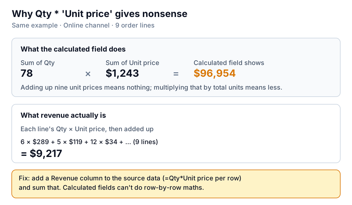
The fix is a column in the source: =[@Qty]*[@[Unit price]] in the table, which the pivot then sums. A calculated field can't do line-by-line arithmetic. Across all 23 lines, the wrong field would claim $1,051,390 of revenue against a real $23,370, so this one is at least easy to spot. The next one isn't.
IF conditions
Say the business pays a 5% bonus on any single order line over $1,000. A calculated field =IF(Revenue>1000, Revenue*0.05, 0) tests the channel's total, not each line:
| Channel | Calculated field (tests the sum) | Per-line rule (correct) |
|---|---|---|
| Market stall | $130.15 | $0.00 |
| Online | $460.85 | $317.90 |
| Wholesale | $577.50 | $541.50 |
| Grand Total | $1,168.50 | $859.40 |
No market-stall line is over $1,000 (the biggest is $510), but the channel's total is $2,603, so the field pays $130.15 that nobody earned. The numbers look plausible, which is what makes this trap dangerous. Any rule about individual transactions belongs in a source column, such as =IF([@Revenue]>1000,[@Revenue]*0.05,0), summed by the pivot.
One more consequence: a calculated field always works from sums, even if you've set Revenue's value field to Average or Count. Changing the summary function of the fields you see doesn't change what the formula receives.
Edit, delete or list a calculated field
- Edit: PivotTable Analyze > Fields, Items & Sets > Calculated Field. Pick the field from the Name drop-down, change the formula, click Modify, then OK.
- Delete: same dialog, pick the name, click Delete. Unticking the field in the Fields pane only hides it; the field stays in the pivot and you can tick it back.
- List all formulas: Fields, Items & Sets > List Formulas writes every calculated field and item, with its formula, to a new sheet. Do this before you hand a workbook to someone else, and keep the sheet as documentation.
- Rename the column heading: Excel shows "Sum of Margin %". Click the heading and type a new name, such as "Margin" (it can't exactly match the field name, so add a space or change a word).
A pivot table calculated field belongs to the pivot cache, so every pivot built from the same source can use it. It updates when you refresh, like any other field; see our guide to refreshing a pivot table if new data isn't showing up.
Calculated field vs calculated item
The same menu has a second option, Calculated Item, and the two are easy to confuse. A calculated field adds a new column of numbers built from other number fields. A calculated item adds a new row label inside an existing field, built from other labels in that field. Microsoft's page notes that formulas for calculated items "operate on the individual records".
| Calculated field | Calculated item | |
|---|---|---|
| Adds | A new value field (e.g. Margin %) | A new item in a row or column field (e.g. Retail) |
| Formula uses | Other fields: =(Revenue - Cost)/Revenue | Items of the same field: =Online + 'Market stall' |
| Where | Fields, Items & Sets > Calculated Field | Select a label in the field first, then > Calculated Item |
| Main risk | Sums first (the traps above) | Counted again in subtotals and totals |
The owner wants a "Retail" line combining Online and the market stall. She selects a Channel label, opens Calculated Item, names it Retail and enters =Online + 'Market stall'. A Retail row appears with $11,820. And the Grand Total jumps to $35,190.
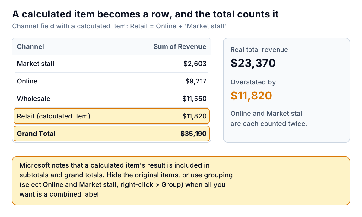
Microsoft's own commission example says the calculated item is included "in the subtotals and grand totals". That's useful for a commission line; it's double counting for a combined label. If you only want Online and Market stall shown together, select both labels, right-click and choose Group: grouping changes the labels without adding money. If you do use a calculated item, filter out the items it combines, and check the Grand Total by hand. Two more limits: you have to ungroup a field before you can add a calculated item to it, and when several calculated items depend on each other, Solve Order on the same menu sets which is worked out first.
When the menu is greyed out, and other limits
If Calculated Field is greyed out, the pivot was almost certainly built with Add this data to the Data Model ticked, or it reads from an OLAP source. Microsoft's page says you can't add calculated fields or items to OLAP-based pivots, and Data Model pivots use measures instead: formulas written in DAX, explained in Microsoft's guide to measures in Power Pivot. A measure for margin, such as =DIVIDE(SUM(Lines[Revenue]) - SUM(Lines[Cost]), SUM(Lines[Revenue])), does the same job and lets you choose the aggregation explicitly. If you don't need the Data Model, rebuilding the pivot without it brings the menu back.
The decision rule for the rest:
- A ratio of totals (margin, average price, cost per unit): calculated field.
- Anything per transaction (Qty × price, IF on a line, a lookup): a column in the source table.
- A combined label: grouping, not a calculated item.
- A distinct count (number of orders rather than lines): the Data Model's Distinct Count, because calculated fields only see sums.
New to pivots? Start with what a pivot table is and how to create one. For the next step after gross margin, our guide to contribution margin shows which costs to take off and why.
If the reason you're adding calculated fields is a monthly margin-by-channel report, consider how much of it you want to maintain by hand. Parity builds a dashboard from your order export or from Shopify, Square or QuickBooks Online directly, with headline numbers, trends, charts and a table of what needs attention. Ratios like margin are worked out from the totals, and every number is checked against queries on the full dataset before you see it. You refine it by chat ("show margin by channel, not by product") and can export it to Excel.
Upload your order lines and get a checked dashboard of revenue, cost and margin for each channel. Build a report from your data free
In Excel, keep the one rule in view: a pivot table calculated field sees sums. Use it for ratios of totals, keep line-level maths in the source, and check one row by hand every time you add a new field.