What you need
Northstar Freight, the example regional logistics distributor we will follow in this guide, closed its monthly billing cycle with a busy shipping calendar across its regional hubs. When the operations lead opened the monthly executive summary tab, the headline revenue card read noticeably lower than the raw invoice export from the accounting software.
Nothing on the summary sheet showed an error flag. Two silent spreadsheet leaks had swallowed a chunk of monthly revenue: an unanchored lookup range stopped short of the new export's bottom rows, and a stale pivot table cache still held the previous month's customer list. A structured formula audit is how you catch both discrepancies before sending the deck to stakeholders.
Before you inspect your first formula or refresh a single cache, gather these items so you can verify every change against a clean baseline:
- The live reporting workbook: Open the multi-tab Excel file or Google Sheet that feeds your stakeholder deck, with edit permissions enabled.
- Fresh raw CSV or Excel exports: Pull unmodified transaction exports directly from your accounting, billing, or CRM tools for the exact reporting period.
- Edit access to pivot table settings: Ensure your permissions allow you to inspect and modify pivot table data source ranges and calculated fields.
- A dedicated control tab: Create a blank worksheet at the front of the file where you will log independent row counts and raw column sums.
1. Prepare a clean snapshot of your workbook and source tabs
Never start fixing formulas inside the only copy of a live monthly workbook. When you overwrite a broken lookup or expand a pivot range, the summary numbers shift immediately, and you lose the trail showing why the previous report was off.
Duplicate the file first and add a control tab at the front of the workbook. Use that tab to record the ground truth from your raw system exports before any lookup or aggregation touches the rows.
Follow these steps to lock in your baseline:
- Freeze a read-only archive copy: Save a timestamped copy of the workbook so you can compare your audited totals against the original broken view.
- Unhide all staging worksheets and columns: Right-click the tab bar and column headers to reveal intermediate helper tabs that often feed executive summaries.
- Record raw row counts and control totals: Sum the primary revenue, cost, and quantity columns directly on the raw export tabs and paste those baseline figures onto your control sheet.
- Standardize tab naming conventions: Remove accidental trailing spaces from worksheet tabs, which frequently break cross-sheet references when a new monthly tab is pasted in.
Tip: Turn on formula view in Excel or Google Sheets by pressing the grave accent shortcut key while holding Control. Scanning a sheet with every cell displaying its underlying syntax makes it easy to spot a lone hard-coded number sitting inside a column of dynamic formulas.
| Audit checkpoint | What to inspect | Common failure mode | Baseline action |
|---|---|---|---|
| Raw export row count | Total rows in CSV vs pasted source tab | Pasted data truncated or appended below lookup range | Log exact row count on control tab |
| Key column data types | Account IDs, SKU codes, and invoice dates | Numbers stored as text or mixed date formats | Run ISTEXT and ISNUMBER checks on keys |
| Worksheet tab names | Exact spelling and spacing of source tabs | Trailing space in new monthly tab breaks sheet references | Strip extra spaces and lock naming pattern |
| Control column sums | Unfiltered SUM of raw revenue and unit columns | Summary tab total drifts from raw transaction sum | Record raw SUM as the target reconciliation figure |
2. Why is VLOOKUP not working when pulling across tabs?
When finance and operations teams ask why a lookup breaks across tabs, the problem is rarely the function name itself. Most cross-tab failures come from three silent shifts: relative table arrays that slide downward as you copy a formula, data type mismatches between tabs, or inserted columns in the source export.
According to Microsoft's VLOOKUP function documentation, omitting the range lookup argument or setting it to TRUE tells the sheet to find an approximate match, which requires the first column to be sorted ascending and returns wrong values on unsorted IDs. For a deeper walkthrough of single-sheet lookup repairs, see our guide on fixing VLOOKUP not working in monthly reports.
How to isolate and repair cross-tab lookup errors
Work through your summary columns in this exact sequence to eliminate false matches and missing rows:
- Force exact matching on every lookup: Check the fourth argument of every legacy lookup and confirm it is set to FALSE, or migrate the column to XLOOKUP where exact match is the default behavior.
- Anchor the external table array: When referencing another tab in VLOOKUP in Google Sheets or Excel, lock the top and bottom row coordinates with dollar signs or reference full columns so new monthly exports never fall outside the box.
- Normalize lookup keys across tabs: Wrap both the lookup value and the source key column in TRIM and VALUE or TEXT functions when one system exports account IDs as text strings and another exports pure integers.
- Replace hard-coded column index numbers: A static third argument breaks the moment an analyst inserts a helper column in the raw data tab, whereas XLOOKUP binds directly to the return column.
| Symptom on summary tab | Root cause across tabs | Excel & Google Sheets fix |
|---|---|---|
| Sudden #N/A on valid rows | Unanchored table array slid down when copied | Lock range coordinates with dollar signs or use structured table references |
| #N/A despite visible key match | Text-formatted ID on one tab vs numeric ID on source tab | Normalize keys with TRIM and TEXT or VALUE before matching |
| Wrong column value returned | Column inserted in source tab shifted static column index | Replace static column number with XLOOKUP return range |
| Plausible but wrong number | Range lookup argument omitted, defaulting to approximate match | Set fourth VLOOKUP argument explicitly to FALSE |
3. Audit SUMIFS and multi-criteria lookups for silent row drops
Lookups that return an error flag at least warn you that a cell needs attention. Multi-criteria aggregations like SUMIFS in Google Sheets and Excel are far more dangerous during a monthly close because a row that fails a filter simply disappears from the total without throwing a warning.
That means a single mistyped category label or unmapped region code silently drops real revenue.
Reconcile multi-criteria summaries against your control total
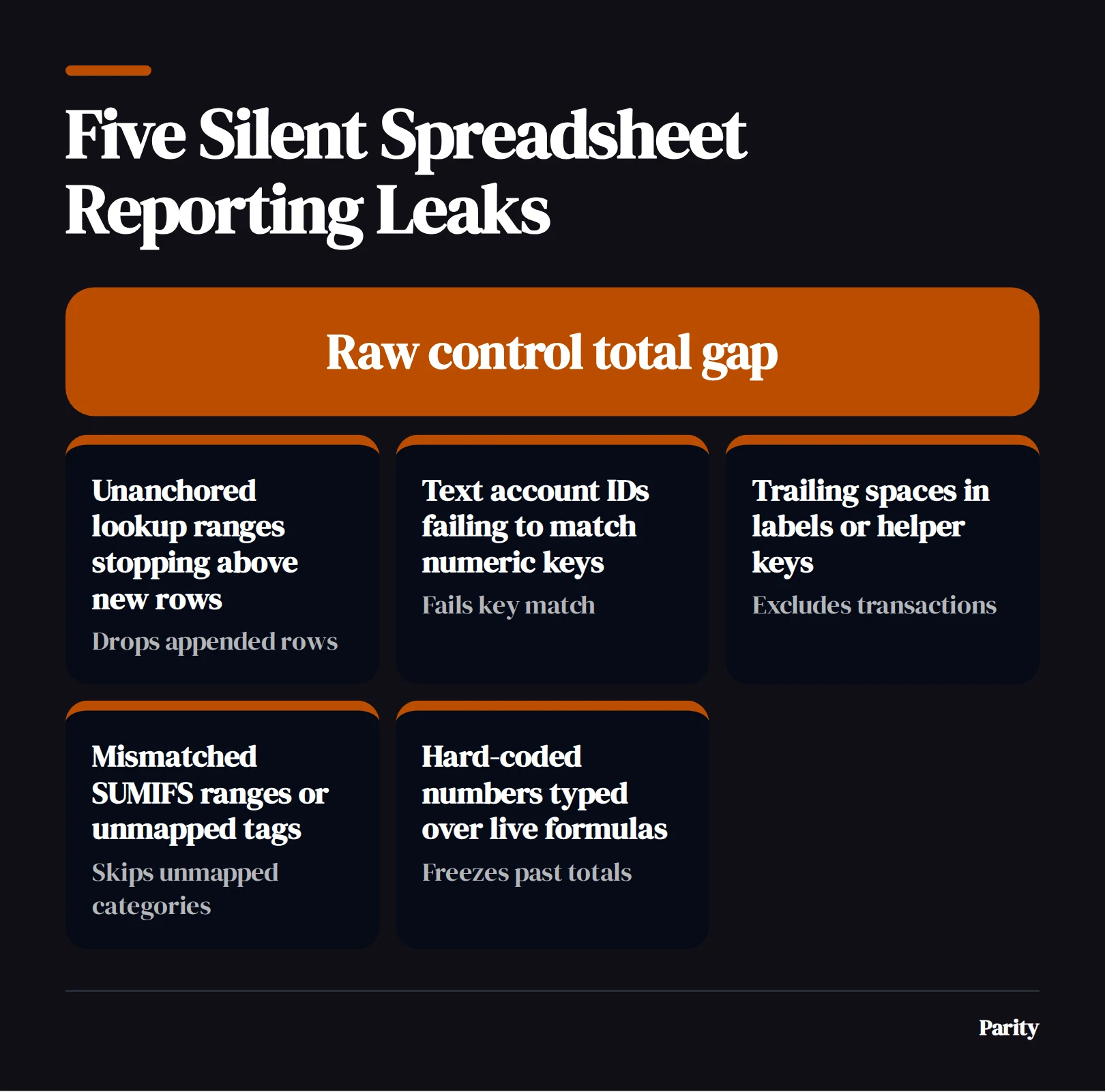
When Northstar Freight audited its regional breakdown table, the individual regional lines added up to less than the raw invoice tab. Use this three-part check to find where rows leak out of multi-criteria tables:
- Verify range symmetry across every argument: Open the formula bar and confirm that the starting and ending row numbers of the sum range match every criteria range down to the last row.
- Test compound lookup keys for hidden spaces: When building a VLOOKUP with multiple criteria using helper columns that concatenate date, region, and SKU, apply TRIM to each component so trailing whitespace in a CRM export does not prevent a match.
- Compare the sum of subsets against the raw total: Add an audit cell below your summary table that subtracts the sum of all category rows from the raw control total, exposing any new category or blank tag that your criteria list missed.
4. How do you refresh a pivot table and verify every total against raw rows?
You can manually refresh a pivot table anytime data changes or set it to refresh automatically when opening the workbook, yet clicking the refresh button only updates the cache from the cell range the pivot table currently knows about.
A pivot table summarizes a specific data range, so adding new rows or columns outside the original static range requires editing the data source range or converting the source data into a dynamic table before refreshing.
If your team pastes a larger month of transactions at the bottom of a raw tab and hits refresh without checking the boundary, every row below the old cutoff is left out of your pivot chart and executive summary. Follow our step-by-step guide on how to refresh a pivot table to update both the source range and the pivot cache cleanly.
Step-by-step pivot table reconciliation
Run this four-step check on every pivot tab before exporting your monthly slides:
- Inspect the source range boundary: Open the Change Data Source dialog in Excel or the data range box in the Google Sheets pivot editor and confirm the bottom row coordinate reaches the final row of your newest export.
- Clear stale filter selections: Check every active row, column, and report filter to ensure a manual checklist selection isn't excluding newly added product lines or sales reps.
- Audit calculated fields and aggregation types: Confirm that value columns are set to Sum rather than Count, which spreadsheets often default to when a single blank cell appears in a numeric column.
- Reconcile the grand total against the control tab: Compare the pivot table's unfiltered grand total directly against the raw column sum you logged in Step 1.
Verify every headline figure directly against source rows
Auditing formulas and pivot caches by hand works, but you have to repeat it every time a fresh CSV lands in the workbook. If you want to skip manual range checks altogether, Parity AI reads spreadsheets across Google Sheets, Excel, and CSV files, reading every row and profiling the columns to build an interactive dashboard and report automatically. Because there are no manual formulas, chart wizards, or data modeling steps to maintain, a pasted export cannot break a cell reference, and every number is verified directly against the underlying source rows.

5. Lock in visual error flags and replace fragile report tabs
Once your lookup columns, multi-criteria tables, and pivot caches reconcile to the cent against your control tab, add permanent visual guardrails so next month's update cannot fail silently. A visible variance banner at the top of your summary sheet saves hours of line-by-line debugging on close day.
Put these three safeguards in place before closing the file:
- Add an automated variance banner: Subtract the summary tab's grand total from the control tab's raw sum, and apply Google Sheets conditional formatting based on another cell or an Excel rule so the cell turns bright red the moment the difference moves away from zero.
- Lock formula columns against accidental edits: Protect all lookup and SUMIFS columns so teammates pasting new transaction data cannot accidentally type a static number over a live formula.
- Document every external tab dependency: Note on your control tab which system exports feed which sheets, along with the exact sort order or key formatting required.
Watch out: Wrapping broken formulas in IFERROR to make ugly error flags disappear hides real data drops. Only use IFERROR when you assign a distinct fallback label such as "Unmapped ID" that you actively count in your control tab.
When your team outgrows fragile multi-tab workbooks, you can move from an Excel to dashboard workflow with an AI dashboard generator. Upload your CSV or Excel files or connect your data sources via read-only access, and Parity AI builds an interactive dashboard and a client-ready report with summaries, charts, tables, and analysis that you can refine in plain English and export to PDF with one click.
Connect Google Sheets or upload an Excel export, and Parity AI builds an interactive dashboard and client-ready report with every number checked against your source rows. Audit your spreadsheet in Parity